
In today's data-driven world, being able to effectively analyze and present data is crucial. One of the most powerful tools for data analysis is Microsoft Excel, and one of its most useful features is the ability to add a second axis to a chart. This feature allows users to display two different data series on the same chart, making it easier to compare and contrast data.
Adding a second axis in Excel on a Mac is a straightforward process that can be completed in a few simple steps.

Why Add a Second Axis in Excel?
There are many reasons why you might want to add a second axis to a chart in Excel. Here are a few:
- Compare different data series: By adding a second axis, you can display two different data series on the same chart, making it easier to compare and contrast data.
- Show different units: If you have two data series with different units, such as dollars and percentages, you can use a second axis to display each series in its own units.
- Highlight trends: A second axis can help to highlight trends in your data that might be difficult to see on a single axis.
How to Add a Second Axis in Excel on a Mac
Adding a second axis in Excel on a Mac is a simple process that can be completed in a few steps.

Step 1: Select the Data Range
First, select the data range that you want to use for your chart. This should include both data series that you want to display on the chart.
Step 2: Create a Chart
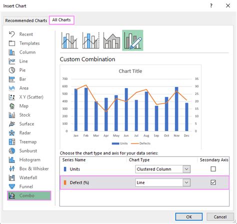
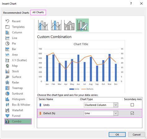
Next, create a chart using the data range that you selected. To do this, go to the "Insert" tab in the ribbon and click on the "Chart" button. Select the type of chart that you want to create, such as a column chart or line chart.
Step 3: Select the Second Data Series
Once you have created your chart, select the second data series that you want to display on the chart. To do this, click on the data series in the chart and then go to the "Chart Design" tab in the ribbon.
Step 4: Add the Second Axis
To add the second axis, click on the "Add Chart Element" button in the "Chart Design" tab. Select "Axes" from the drop-down menu and then select "Secondary Axis".

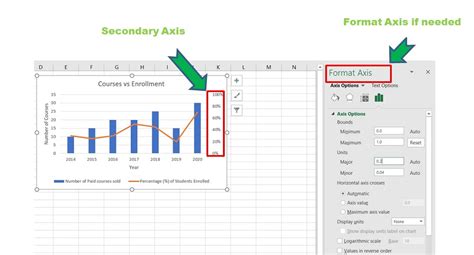
Step 5: Customize the Second Axis
Once you have added the second axis, you can customize it to suit your needs. To do this, click on the second axis in the chart and then go to the "Format Axis" tab in the ribbon. From here, you can change the axis title, labels, and other settings.
Tips and Variations
Here are a few tips and variations to keep in mind when adding a second axis in Excel on a Mac:
- Use different chart types: Depending on the type of data you are working with, you may want to use a different type of chart. For example, if you are working with time-based data, a line chart may be a good choice.
- Customize the axis labels: You can customize the axis labels to make your chart more readable. To do this, click on the axis labels and then go to the "Format Axis" tab in the ribbon.
- Use a secondary axis title: You can add a title to the secondary axis to make it clear what the axis represents. To do this, click on the secondary axis and then go to the "Format Axis" tab in the ribbon.
Second Axis in Excel Image Gallery


Conclusion
Adding a second axis in Excel on a Mac is a simple process that can help to enhance your charts and make your data more readable. By following the steps outlined above, you can easily add a second axis to your charts and customize it to suit your needs. Whether you are working with financial data, scientific data, or any other type of data, a second axis can help to make your charts more informative and engaging.