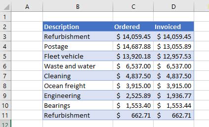
Alternate Row Color In Google Sheets Made Easy

Alternate row coloring, also known as zebra striping, is a formatting technique used in Google Sheets to make data easier to read by alternating the background color of rows. This technique is particularly useful when working with large datasets, as it helps to visually distinguish one row from another.

In this article, we will explore the different methods to achieve alternate row coloring in Google Sheets, including using formulas, conditional formatting, and Google Sheets add-ons.

Method 1: Using Formulas

One way to achieve alternate row coloring in Google Sheets is by using formulas. You can use the ISEVEN or ISODD function to check if a row number is even or odd, and then use the IF function to apply a specific background color.

Here's an example formula:

=ISEVEN(ROW(A1))

Assuming you want to apply the background color to cell A1, you can use the following formula:

=IF(ISEVEN(ROW(A1)), "highlight", "")

Then, select the entire range of cells you want to format, go to the "Format" tab, select "Conditional formatting," and enter the formula.

Step-by-Step Instructions:

1. Select the entire range of cells you want to format.
2. Go to the "Format" tab.
3. Select "Conditional formatting."
4. Enter the formula =ISEVEN(ROW(A1)).
5. Choose a background color.
6. Click "Done."

Method 2: Using Conditional Formatting

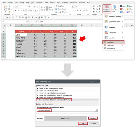
Another way to achieve alternate row coloring in Google Sheets is by using conditional formatting. You can use the "Custom formula" option in the conditional formatting rules to apply a background color to every other row.

Here's how:

1. Select the entire range of cells you want to format.
2. Go to the "Format" tab.
3. Select "Conditional formatting."
4. Choose "Custom formula."
5. Enter the formula =ISEVEN(ROW(A1)).
6. Choose a background color.
7. Click "Done."

Customizing the Formula:

You can customize the formula to start the alternate row coloring from a specific row or to apply the formatting to a specific range of cells.

For example, to start the alternate row coloring from row 3, you can use the following formula:

=ISEVEN(ROW(A3)-2)

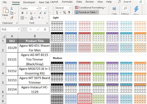
Method 3: Using Google Sheets Add-ons

If you want a more straightforward way to achieve alternate row coloring in Google Sheets, you can use add-ons like "Format Tools" or "Table Formatter."

Here's how to use the "Format Tools" add-on:

1. Install the "Format Tools" add-on from the Google Workspace Marketplace.
2. Select the entire range of cells you want to format.
3. Go to the "Format" tab.
4. Click on the "Format Tools" icon.
5. Select "Alternate row coloring."
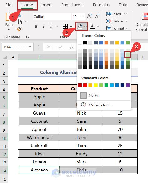
6. Choose a background color.
7. Click "Apply."

Benefits of Using Add-ons:

Using add-ons can save you time and effort, as they provide a simple and intuitive way to apply formatting to your data.

Method 4: Using a Script

If you're comfortable with scripting, you can use Google Apps Script to achieve alternate row coloring in Google Sheets.

Here's an example script:

function onOpen() {
  var sheet = SpreadsheetApp.getActiveSpreadsheet().getActiveSheet();
  var range = sheet.getDataRange();
  var rows = range.getNumRows();
  
  for (var i = 1; i <= rows; i++) {
    if (i % 2 == 0) {
      sheet.getRange(i, 1, 1, range.getNumColumns()).setBackground("highlight");
    }
  }
}

Step-by-Step Instructions:

1. Open the Google Apps Script editor by clicking on "Tools" > "Script editor."
2. Delete any existing code in the editor.
3. Paste the script into the editor.
4. Save the script by clicking on the floppy disk icon or pressing Ctrl+S (or Cmd+S on a Mac).
5. Go back to your Google Sheet and refresh the page.

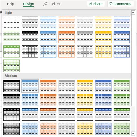
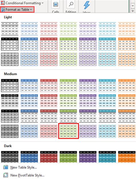
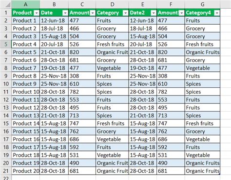
Gallery of Alternate Row Color Examples:

Alternate Row Color Examples

We hope this article has helped you to achieve alternate row coloring in Google Sheets using different methods. Whether you prefer using formulas, conditional formatting, or add-ons, there's a method that suits your needs.

If you have any questions or need further assistance, please don't hesitate to comment below. We'd be happy to help!

Also, if you found this article helpful, please share it with your friends and colleagues who might benefit from it.