Intro
The binomial pricing model is a widely used method for valuing options, particularly American-style options that can be exercised before expiration. While it may seem daunting, creating a binomial pricing model in Excel can be made easy with a few simple steps. In this article, we will break down the process into manageable parts, making it accessible to readers of all levels.
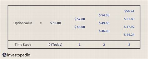
The binomial pricing model is a discrete-time model, which means that it assumes that time is divided into discrete intervals, rather than being continuous. This allows us to model the behavior of the underlying asset price over time, using a series of up and down movements. The model is based on the idea that the price of the underlying asset can only move in one of two directions at each time step: up or down.
Understanding the Binomial Pricing Model
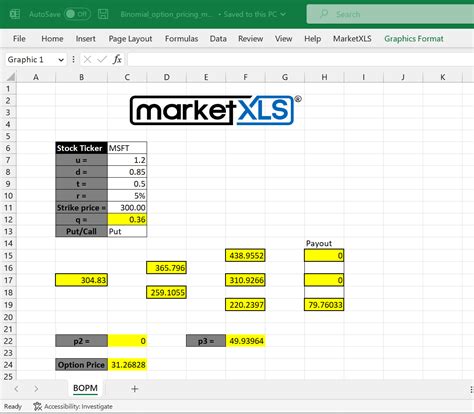
Before we dive into creating the model in Excel, let's take a step back and understand the underlying mathematics. The binomial pricing model is based on the following assumptions:
- The price of the underlying asset can only move up or down at each time step
- The probability of an up move is p, and the probability of a down move is 1-p
- The size of the up and down moves is constant over time
- The risk-free interest rate is constant over time
Using these assumptions, we can calculate the value of the option at each node in the lattice, using the following formula:
C = max(S-K,0)
Where:
- C is the value of the call option
- S is the price of the underlying asset
- K is the strike price
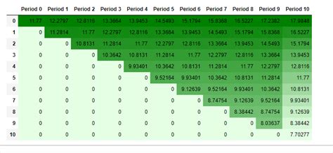
We can then use the risk-neutral probabilities to calculate the expected value of the option at each node, and work backwards through the lattice to find the value of the option today.
Creating the Binomial Pricing Model in Excel
Now that we have a solid understanding of the underlying mathematics, let's create the binomial pricing model in Excel. We will use the following inputs:
- S: the current price of the underlying asset
- K: the strike price
- T: the time to expiration
- r: the risk-free interest rate
- σ: the volatility of the underlying asset
We will also use the following formulas to calculate the size of the up and down moves:
u = exp(σ√Δt) d = 1/u
Where:
- u is the size of the up move
- d is the size of the down move
- Δt is the time step
We can then use the following formula to calculate the risk-neutral probabilities:
p = (exp(rΔt) - d) / (u - d)
Using these inputs and formulas, we can create the binomial pricing model in Excel.
Step-by-Step Guide to Creating the Binomial Pricing Model in Excel

Here is a step-by-step guide to creating the binomial pricing model in Excel:
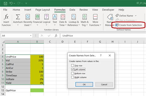
- Set up the inputs: Create a table with the inputs, including the current price of the underlying asset, the strike price, the time to expiration, the risk-free interest rate, and the volatility of the underlying asset.
- Calculate the size of the up and down moves: Use the formulas above to calculate the size of the up and down moves.
- Calculate the risk-neutral probabilities: Use the formula above to calculate the risk-neutral probabilities.
- Create the lattice: Use the inputs and formulas to create the lattice, using a combination of IF statements and VLOOKUPs to calculate the value of the option at each node.
- Calculate the value of the option: Use the lattice to calculate the value of the option, working backwards through the lattice to find the value of the option today.
Example of a Binomial Pricing Model in Excel
Here is an example of a binomial pricing model in Excel:
| A | B | C | D | E | F | G | |
|---|---|---|---|---|---|---|---|
| 1 | S | 100 | |||||
| 2 | K | 120 | |||||
| 3 | T | 1 | |||||
| 4 | r | 0.05 | |||||
| 5 | σ | 0.2 | |||||
| 6 | u | =exp($E$5*sqrt($E$3/100)) | |||||
| 7 | d | =1/$E$6 | |||||
| 8 | p | =(exp($E$4*$E$3/100)-$E$7)/($E$6-$E$7) |
| H | I | J | K | L | M | N | |
|---|---|---|---|---|---|---|---|
| 9 | 100 | 120 | 144 | ||||
| 10 | 80 | 100 | 120 | ||||
| 11 | 64 | 80 | 100 | ||||
| 12 |
In this example, the binomial pricing model is used to value a call option with a strike price of 120 and a time to expiration of 1 year. The underlying asset price is assumed to be 100, and the risk-free interest rate is assumed to be 5%. The volatility of the underlying asset is assumed to be 20%.
Advantages and Limitations of the Binomial Pricing Model
The binomial pricing model has several advantages, including:
- It is a simple and intuitive model that is easy to understand and implement
- It can be used to value American-style options, which can be exercised before expiration
- It can be used to value options with complex payoffs, such as barrier options and binary options
However, the binomial pricing model also has several limitations, including:
- It is a discrete-time model, which means that it assumes that time is divided into discrete intervals, rather than being continuous
- It assumes that the price of the underlying asset can only move in one of two directions at each time step, rather than being able to move continuously
- It assumes that the risk-free interest rate and volatility of the underlying asset are constant over time, rather than being able to change over time.
Conclusion
In conclusion, the binomial pricing model is a powerful tool for valuing options, particularly American-style options that can be exercised before expiration. While it may seem daunting, creating a binomial pricing model in Excel can be made easy with a few simple steps. By following the steps outlined in this article, readers can create their own binomial pricing model in Excel and start valuing options today.
We hope this article has provided you with a comprehensive understanding of the binomial pricing model and how to create it in Excel. If you have any questions or comments, please don't hesitate to reach out.
Binomial Pricing Model Image Gallery


