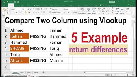
Comparing values in two Excel columns is a common task that can be accomplished in several ways. Whether you're working with a small dataset or a large one, Excel provides various methods to compare columns, making it easier to identify similarities, differences, and patterns. In this article, we'll explore the different ways to compare values in two Excel columns, including formulas, conditional formatting, and other techniques.

Why Compare Values in Two Excel Columns?
Comparing values in two Excel columns can help you:
- Identify duplicate values
- Find unique values
- Highlight differences between two datasets
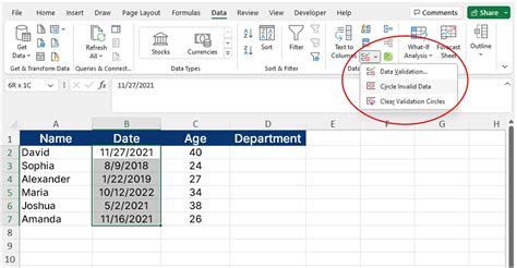
- Perform data validation
- Create reports and summaries
Method 1: Using the IF Function
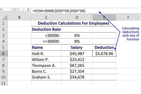
One of the simplest ways to compare values in two Excel columns is by using the IF function. The syntax for the IF function is:
IF(logical_test, [value_if_true], [value_if_false])
For example, suppose you want to compare the values in columns A and B, and return "Match" if the values are the same, and "No Match" if they're different. You can use the following formula:
=IF(A2=B2, "Match", "No Match")
Assuming the values you want to compare are in cells A2 and B2.
Method 2: Using the VLOOKUP Function
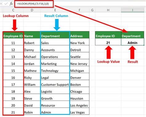
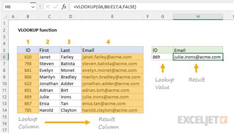
Another way to compare values in two Excel columns is by using the VLOOKUP function. The syntax for the VLOOKUP function is:
VLOOKUP(lookup_value, table_array, col_index_num, [range_lookup])
For example, suppose you want to look up the value in cell A2 in column B, and return the corresponding value in column C. You can use the following formula:
=VLOOKUP(A2, B:C, 2, FALSE)
Assuming the values you want to look up are in column B, and the corresponding values are in column C.
Method 3: Using Conditional Formatting
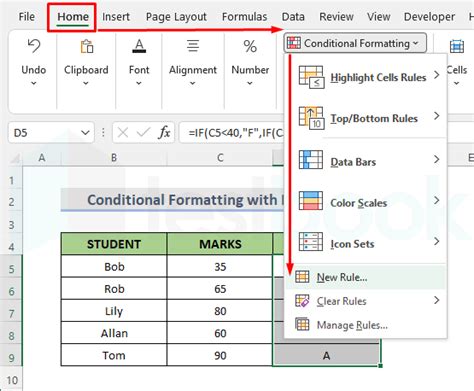
Conditional formatting is a powerful tool in Excel that allows you to highlight cells based on specific conditions. You can use conditional formatting to compare values in two Excel columns and highlight the differences.
To use conditional formatting, select the cells you want to format, go to the Home tab, and click on the Conditional Formatting button. Then, select "New Rule" and choose "Use a formula to determine which cells to format".
For example, suppose you want to highlight the cells in column A that are different from the cells in column B. You can use the following formula:
=A2<>B2
Assuming the values you want to compare are in cells A2 and B2.
Method 4: Using the Filter Function
The Filter function is another way to compare values in two Excel columns. The Filter function allows you to filter a range of cells based on specific conditions.
To use the Filter function, select the cells you want to filter, go to the Data tab, and click on the Filter button. Then, select "Filter" and choose the condition you want to apply.
For example, suppose you want to filter the cells in column A that are different from the cells in column B. You can use the following formula:
=FILTER(A:A, A:A<>B:B)
Assuming the values you want to compare are in columns A and B.

Method 5: Using Power Query
Power Query is a powerful tool in Excel that allows you to manipulate and analyze data. You can use Power Query to compare values in two Excel columns and perform various operations.
To use Power Query, go to the Data tab, and click on the "From Other Sources" button. Then, select "Blank Query" and choose the range of cells you want to compare.
For example, suppose you want to compare the values in columns A and B, and return the differences. You can use the following formula:
= Table.Combine({Table1, Table2}, {"Column1", "Column2"}, JoinKind.Inner)
Assuming the values you want to compare are in tables Table1 and Table2.

Conclusion
Comparing values in two Excel columns is a common task that can be accomplished in several ways. Whether you're using formulas, conditional formatting, or other techniques, Excel provides various methods to compare columns and identify similarities, differences, and patterns.
In this article, we've explored five different methods to compare values in two Excel columns, including the IF function, VLOOKUP function, conditional formatting, Filter function, and Power Query. Each method has its own strengths and weaknesses, and the choice of method depends on the specific task and dataset.
We hope this article has helped you learn how to compare values in two Excel columns easily and efficiently. Do you have any other questions about comparing values in Excel? Share your thoughts and comments below!
Gallery of Excel Comparison Techniques
Excel Comparison Techniques
