5 Ways To Use Conditional Formatting In Excel For Yes/No Cells

Using conditional formatting in Excel can greatly enhance the visual appeal and functionality of your spreadsheets. One common scenario where conditional formatting is particularly useful is when working with yes/no cells, also known as Boolean values. In this article, we'll explore five ways to use conditional formatting to make the most out of your yes/no cells in Excel.

Why Use Conditional Formatting for Yes/No Cells?

Before we dive into the specific techniques, it's essential to understand why conditional formatting is beneficial for yes/no cells. By applying conditional formatting, you can:

Visually distinguish between yes and no values, making it easier to scan and analyze data
Highlight important information, such as errors or inconsistencies
Create interactive dashboards and reports that respond to user input
Enhance the overall readability and professionalism of your spreadsheets

Method 1: Simple Yes/No Highlighting

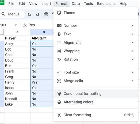
One of the most basic yet effective ways to use conditional formatting for yes/no cells is to highlight the cells based on their values. To do this:

Select the range of cells containing the yes/no values
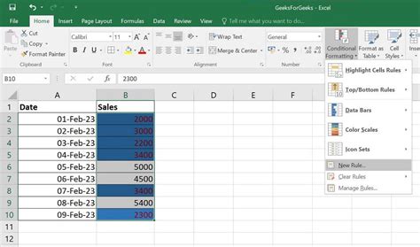
Go to the Home tab in the Excel ribbon
Click on the Conditional Formatting button in the Styles group
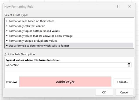
Select "New Rule"
Choose "Use a formula to determine which cells to format"
Enter the formula =A1="Yes" (assuming the yes/no values are in column A)
Click on the Format button and select a fill color, such as green
Click OK

Repeat the process for the "No" values by entering the formula =A1="No" and selecting a different fill color, such as red.

Conditional Formatting Yes No Cells Simple Highlighting

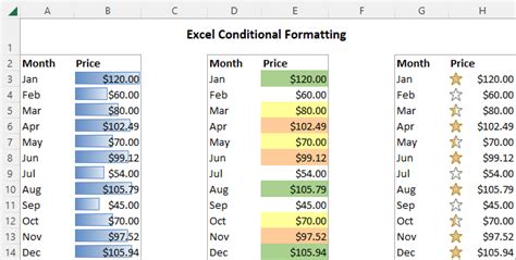
Method 2: Icon Sets for Yes/No Values

Another way to visually distinguish between yes and no values is to use icon sets. Excel provides a variety of icon sets that can be used to represent different values.

Select the range of cells containing the yes/no values
Go to the Home tab in the Excel ribbon
Click on the Conditional Formatting button in the Styles group
Select "Icon Sets"
Choose a suitable icon set, such as the "Ticks and Crosses" set
Click OK

Excel will automatically apply the icon set to the cells based on their values.

Conditional Formatting Yes No Cells Icon Sets

Method 3: Data Bars for Yes/No Progress

Data bars can be used to create a progress bar effect for yes/no values. This is particularly useful when tracking the completion of tasks or projects.

Select the range of cells containing the yes/no values
Go to the Home tab in the Excel ribbon
Click on the Conditional Formatting button in the Styles group
Select "Data Bars"
Choose a suitable data bar style
Click OK

Excel will apply the data bar to the cells based on their values.

Conditional Formatting Yes No Cells Data Bars

Method 4: Color Scales for Yes/No Ranges

Color scales can be used to create a gradient effect for yes/no values. This is particularly useful when tracking the progress of multiple tasks or projects.

Select the range of cells containing the yes/no values
Go to the Home tab in the Excel ribbon
Click on the Conditional Formatting button in the Styles group
Select "Color Scales"
Choose a suitable color scale
Click OK

Excel will apply the color scale to the cells based on their values.

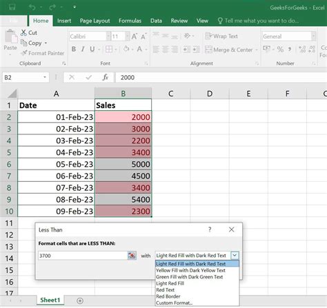
Conditional Formatting Yes No Cells Color Scales

Method 5: Formula-Based Formatting

The final method involves using a formula to determine the formatting of the cells. This is particularly useful when you need to apply complex logic to your formatting rules.

Select the range of cells containing the yes/no values
Go to the Home tab in the Excel ribbon
Click on the Conditional Formatting button in the Styles group
Select "New Rule"
Choose "Use a formula to determine which cells to format"
Enter a formula that evaluates the yes/no values, such as =IF(A1="Yes",TRUE,FALSE)
Click on the Format button and select a fill color or other formatting options
Click OK

Excel will apply the formatting based on the formula.

Conditional Formatting Yes No Cells Formula-Based Formatting

Gallery of Conditional Formatting Examples

Conditional Formatting Examples

Take Your Conditional Formatting to the Next Level

In this article, we've explored five ways to use conditional formatting to enhance the visual appeal and functionality of your yes/no cells in Excel. Whether you're looking to create a simple highlighting effect or a complex formula-based formatting rule, conditional formatting has got you covered. Experiment with different techniques and formulas to take your conditional formatting to the next level.