
Conditional formatting in Google Sheets is a powerful tool that allows you to highlight cells based on specific conditions or rules. This feature helps to draw attention to important information, trends, and patterns in your data, making it easier to analyze and understand. In this article, we will explore five ways to apply conditional formatting in Google Sheets, along with practical examples and step-by-step instructions.
What is Conditional Formatting?
Conditional formatting is a feature in Google Sheets that allows you to apply formatting to cells based on specific conditions or rules. This can include highlighting cells that contain specific values, formatting cells based on formulas, or creating custom rules using Google Sheets functions.
Method 1: Highlight Cells Based on Value

One of the most common uses of conditional formatting is to highlight cells based on their value. For example, you might want to highlight all cells that contain a specific value, such as "Yes" or "No". To do this, follow these steps:
- Select the range of cells you want to format.
- Go to the "Format" tab in the top menu.
- Select "Conditional formatting".
- In the "Format cells if" dropdown menu, select "Value".
- Enter the value you want to highlight, such as "Yes" or "No".
- Choose a formatting option, such as fill color or font color.
- Click "Done".
Example: Highlighting Sales Over $1000
Suppose you have a spreadsheet that contains sales data, and you want to highlight all sales over $1000. To do this, follow these steps:
- Select the range of cells that contains the sales data.
- Go to the "Format" tab in the top menu.
- Select "Conditional formatting".
- In the "Format cells if" dropdown menu, select "Value".
- Enter the value "1000" in the " Greater than" field.
- Choose a formatting option, such as fill color or font color.
- Click "Done".
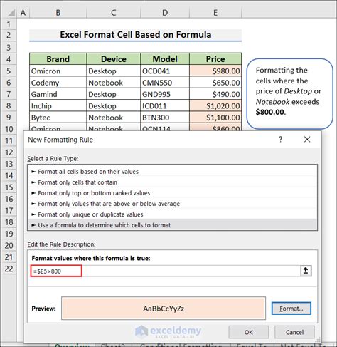
Method 2: Format Cells Based on Formula

Conditional formatting can also be used to format cells based on formulas. For example, you might want to highlight cells that contain a specific formula or value. To do this, follow these steps:
- Select the range of cells you want to format.
- Go to the "Format" tab in the top menu.
- Select "Conditional formatting".
- In the "Format cells if" dropdown menu, select "Custom formula is".
- Enter the formula you want to use to format the cells.
- Choose a formatting option, such as fill color or font color.
- Click "Done".
Example: Highlighting Cells with a Specific Formula
Suppose you have a spreadsheet that contains a formula to calculate the total sales, and you want to highlight all cells that contain this formula. To do this, follow these steps:
- Select the range of cells that contains the formula.
- Go to the "Format" tab in the top menu.
- Select "Conditional formatting".
- In the "Format cells if" dropdown menu, select "Custom formula is".
- Enter the formula
=SUM(A1:A10)in the "Custom formula is" field. - Choose a formatting option, such as fill color or font color.
- Click "Done".
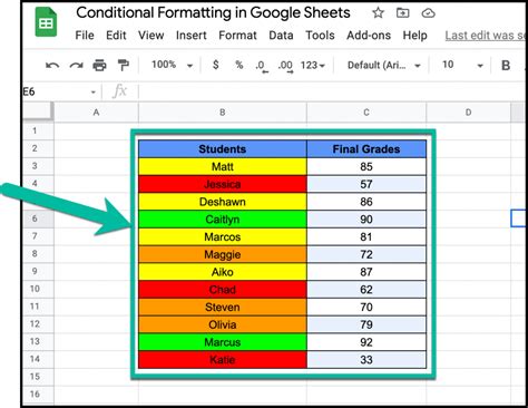
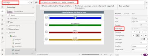
Method 3: Create Custom Rules Using Google Sheets Functions

Google Sheets provides a range of functions that can be used to create custom rules for conditional formatting. For example, you can use the IF function to highlight cells based on a specific condition. To do this, follow these steps:
- Select the range of cells you want to format.
- Go to the "Format" tab in the top menu.
- Select "Conditional formatting".
- In the "Format cells if" dropdown menu, select "Custom formula is".
- Enter the formula you want to use to format the cells, using a Google Sheets function such as
IF. - Choose a formatting option, such as fill color or font color.
- Click "Done".
Example: Highlighting Cells with a Specific Condition
Suppose you have a spreadsheet that contains data on student grades, and you want to highlight all cells that contain a grade of "A" or "B". To do this, follow these steps:
- Select the range of cells that contains the grades.
- Go to the "Format" tab in the top menu.
- Select "Conditional formatting".
- In the "Format cells if" dropdown menu, select "Custom formula is".
- Enter the formula
=IF(A1:A10="A",TRUE,FALSE)in the "Custom formula is" field. - Choose a formatting option, such as fill color or font color.
- Click "Done".
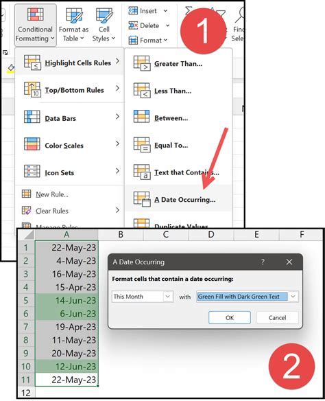
Method 4: Format Cells Based on Date
Conditional formatting can also be used to format cells based on dates. For example, you might want to highlight all cells that contain a specific date or range of dates. To do this, follow these steps:
- Select the range of cells you want to format.
- Go to the "Format" tab in the top menu.
- Select "Conditional formatting".
- In the "Format cells if" dropdown menu, select "Date".
- Enter the date or range of dates you want to highlight.
- Choose a formatting option, such as fill color or font color.
- Click "Done".
Example: Highlighting Cells with a Specific Date
Suppose you have a spreadsheet that contains data on event dates, and you want to highlight all cells that contain a specific date, such as "2022-02-14". To do this, follow these steps:
- Select the range of cells that contains the dates.
- Go to the "Format" tab in the top menu.
- Select "Conditional formatting".
- In the "Format cells if" dropdown menu, select "Date".
- Enter the date "2022-02-14" in the "Date" field.
- Choose a formatting option, such as fill color or font color.
- Click "Done".
Method 5: Format Cells Based on Text
Conditional formatting can also be used to format cells based on text. For example, you might want to highlight all cells that contain a specific text string. To do this, follow these steps:
- Select the range of cells you want to format.
- Go to the "Format" tab in the top menu.
- Select "Conditional formatting".
- In the "Format cells if" dropdown menu, select "Text".
- Enter the text string you want to highlight.
- Choose a formatting option, such as fill color or font color.
- Click "Done".
Example: Highlighting Cells with a Specific Text String
Suppose you have a spreadsheet that contains data on customer feedback, and you want to highlight all cells that contain the text string "Excellent". To do this, follow these steps:
- Select the range of cells that contains the feedback.
- Go to the "Format" tab in the top menu.
- Select "Conditional formatting".
- In the "Format cells if" dropdown menu, select "Text".
- Enter the text string "Excellent" in the "Text" field.
- Choose a formatting option, such as fill color or font color.
- Click "Done".
Conditional Formatting Image Gallery


We hope this article has provided you with a comprehensive guide to applying conditional formatting in Google Sheets. Whether you're a beginner or an advanced user, these methods can help you to create powerful and informative spreadsheets that showcase your data in a meaningful way. Try out these methods and experiment with different formatting options to get the most out of your data.
We encourage you to share your experiences and tips for using conditional formatting in Google Sheets in the comments below. What are some creative ways you've used conditional formatting in your own spreadsheets?