
The art of formatting in Google Sheets! Formatting a whole row can be a tedious task, but don't worry, we've got you covered. In this article, we'll explore the easiest ways to format a whole row in Google Sheets, making your spreadsheet look professional and easy to read.
Why Format a Whole Row in Google Sheets?
Formatting a whole row in Google Sheets can help:
- Highlight important information
- Create visual hierarchy
- Improve readability
- Enhance the overall appearance of your spreadsheet
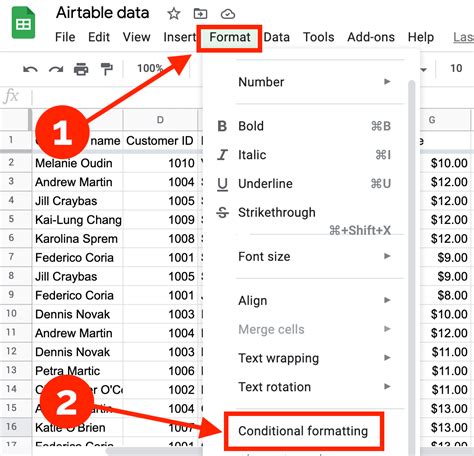
Method 1: Using the Format Tab
The most straightforward way to format a whole row is by using the Format tab. Here's how:
- Select the row you want to format by clicking on the row number.
- Go to the Format tab in the top menu.
- Choose the format you want to apply, such as font color, background color, or borders.
- Select the format options and click Apply.
This method is quick and easy, but it only allows you to apply basic formats.
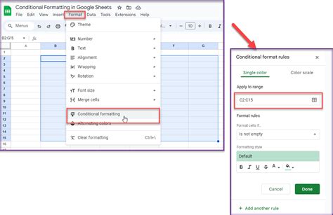
Method 2: Using Conditional Formatting
Conditional formatting allows you to format a whole row based on specific conditions. Here's how:
- Select the row you want to format.
- Go to the Format tab and select Conditional formatting.
- Choose the condition you want to apply, such as "if cell contains" or "if cell is greater than".
- Set the condition rules and select the format options.
- Click Done.
This method is more powerful than the previous one, as it allows you to format a whole row based on specific conditions.
Method 3: Using Google Sheets Formulas
You can also use Google Sheets formulas to format a whole row. Here's how:
- Select the row you want to format.
- Enter a formula in the first cell of the row, such as
=IF(A1>0,"Format this row"). - Press Enter to apply the formula.
- Select the format options and click Apply.
This method is more advanced, but it allows you to format a whole row based on complex conditions.
Method 4: Using Google Sheets Scripts
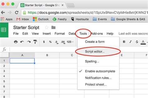
If you want to automate the formatting process, you can use Google Sheets scripts. Here's how:
- Open the Google Apps Script editor by clicking on Tools > Script editor.
- Write a script that formats the whole row, such as
function formatRow() { var sheet = SpreadsheetApp.getActiveSheet(); sheet.getRange("A1:Z1").setFontColor("red"); }. - Save the script and click on the Run button.
This method is more advanced, but it allows you to automate the formatting process.
Tips and Tricks
- To format multiple rows, select the rows you want to format and apply the format options.
- To format a whole column, select the column header and apply the format options.
- To undo a format, go to the Edit menu and select Undo.
- To redo a format, go to the Edit menu and select Redo.
Conclusion
Formatting a whole row in Google Sheets is easy and can enhance the appearance of your spreadsheet. By using the Format tab, conditional formatting, formulas, or scripts, you can create a professional-looking spreadsheet that's easy to read. Try out these methods and take your spreadsheet formatting skills to the next level!
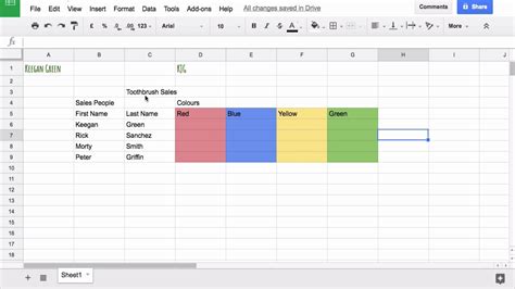
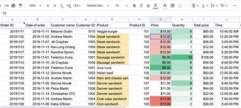
Gallery of Google Sheets Formatting Examples


We hope this article has helped you learn how to format a whole row in Google Sheets. If you have any questions or need further assistance, please don't hesitate to ask. Happy formatting!