5 Ways To Color By Number In Excel

Excel is an incredibly powerful tool for data analysis, and one of its many features is the ability to color cells based on specific conditions. Color by number, also known as conditional formatting, is a popular technique used to highlight cells that meet certain criteria, making it easier to visualize and understand complex data. In this article, we'll explore five ways to color by number in Excel, providing you with a comprehensive guide to enhance your spreadsheet skills.

Color by number is a fundamental aspect of data visualization, allowing you to quickly identify trends, patterns, and outliers in your data. By applying different colors to cells based on their values, you can create a more engaging and informative spreadsheet that helps you make better decisions.

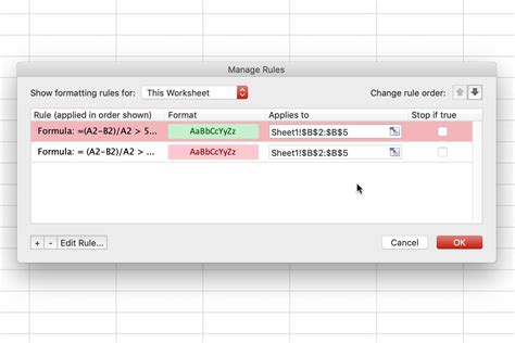
Method 1: Using Conditional Formatting Rules

One of the most common ways to color by number in Excel is by using conditional formatting rules. This method allows you to create specific rules that determine which cells to format based on their values. To access conditional formatting rules, follow these steps:

1. Select the cells you want to format.
2. Go to the "Home" tab in the Excel ribbon.
3. Click on the "Conditional Formatting" button in the "Styles" group.
4. Choose "New Rule" from the dropdown menu.
5. Select the type of rule you want to create (e.g., "Format only cells that contain").
6. Define the condition and format.
7. Click "OK" to apply the rule.

Types of Conditional Formatting Rules

Excel offers several types of conditional formatting rules, including:

• Format only cells that contain
• Format only top or bottom ranked values
• Format only values that are above or below average
• Format only unique or duplicate values
• Use a formula to determine which cells to format

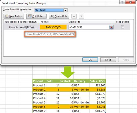
Method 2: Using Formulas and Conditional Formatting

Another way to color by number in Excel is by using formulas in conjunction with conditional formatting. This method provides more flexibility and allows you to create custom conditions based on your data. To use formulas and conditional formatting, follow these steps:

1. Select the cells you want to format.
2. Go to the "Home" tab in the Excel ribbon.
3. Click on the "Conditional Formatting" button in the "Styles" group.
4. Choose "New Rule" from the dropdown menu.
5. Select "Use a formula to determine which cells to format."
6. Enter your formula in the "Format values where this formula is true" field.
7. Define the format.
8. Click "OK" to apply the rule.

Examples of Formulas for Conditional Formatting

Some examples of formulas you can use for conditional formatting include:

• =A1>10 to format cells in column A that are greater than 10
• =B1<5 to format cells in column B that are less than 5
• =C1=C2 to format cells in column C that are equal to the value in cell C2

Method 3: Using Color Scales and Icon Sets

Color scales and icon sets are pre-built formatting options in Excel that allow you to quickly color cells based on their values. To use color scales and icon sets, follow these steps:

1. Select the cells you want to format.
2. Go to the "Home" tab in the Excel ribbon.
3. Click on the "Conditional Formatting" button in the "Styles" group.
4. Choose "Color Scales" or "Icon Sets" from the dropdown menu.
5. Select the desired color scale or icon set.
6. Click "OK" to apply the formatting.

Types of Color Scales and Icon Sets

Excel offers several types of color scales and icon sets, including:

• Color scales (e.g., red, yellow, green)
• Icon sets (e.g., arrows, flags, stars)

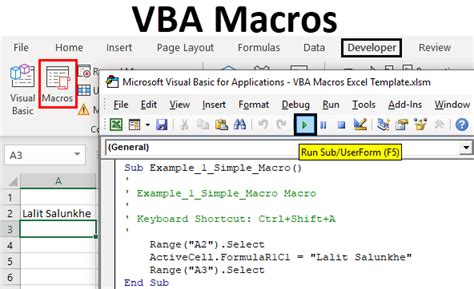
Method 4: Using VBA Macros

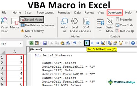
VBA macros are a powerful way to automate tasks in Excel, including color by number formatting. To use VBA macros, follow these steps:

1. Open the Visual Basic Editor by pressing "Alt + F11" or by navigating to "Developer" > "Visual Basic" in the Excel ribbon.
2. Create a new module by clicking "Insert" > "Module" in the Visual Basic Editor.
3. Write your VBA code to color cells based on their values.
4. Save the module and return to your Excel spreadsheet.
5. Run the macro by clicking "Developer" > "Macros" in the Excel ribbon.

Example VBA Code for Color by Number

Here's an example VBA code that colors cells in column A based on their values:

Sub ColorByNumber()
    Dim cell As Range
    For Each cell In Range("A1:A10")
        If cell.Value > 10 Then
            cell.Interior.Color = vbRed
        ElseIf cell.Value < 5 Then
            cell.Interior.Color = vbGreen
        End If
    Next cell
End Sub

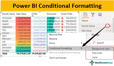
Method 5: Using Power Query and Conditional Formatting

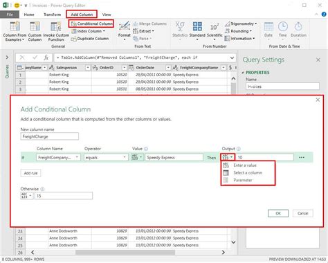
Power Query is a powerful data manipulation tool in Excel that allows you to color cells based on their values using conditional formatting. To use Power Query and conditional formatting, follow these steps:

1. Select the cells you want to format.
2. Go to the "Data" tab in the Excel ribbon.
3. Click on the "From Table/Range" button in the "Get & Transform Data" group.
4. Create a new query by clicking "OK" in the "Create Table" dialog box.
5. Apply conditional formatting to the query by clicking "Home" > "Conditional Formatting" in the Power Query Editor.
6. Define the condition and format.
7. Click "OK" to apply the rule.

Benefits of Using Power Query and Conditional Formatting

Using Power Query and conditional formatting provides several benefits, including:

• Improved data visualization
• Enhanced data analysis
• Increased productivity

Color by Number Image Gallery

In conclusion, color by number is a powerful technique in Excel that allows you to visualize and analyze complex data. By using one of the five methods outlined in this article, you can enhance your spreadsheet skills and make better decisions. Remember to experiment with different techniques and formulas to find the best approach for your specific needs.