Cells are the basic building blocks of any Excel spreadsheet, and comparing them is a common task that many users face. Whether you're tracking changes, identifying duplicates, or verifying data, comparing cells in Excel is an essential skill to master. In this article, we'll explore five ways to compare cells in Excel, including using formulas, conditional formatting, and more.
Understanding the Basics of Cell Comparison
Before we dive into the methods, it's essential to understand the basics of cell comparison in Excel. When comparing cells, you can use various operators, such as =, <, >, <=, >=, and <>. These operators help you identify similarities and differences between cells.
Method 1: Using the IF Function
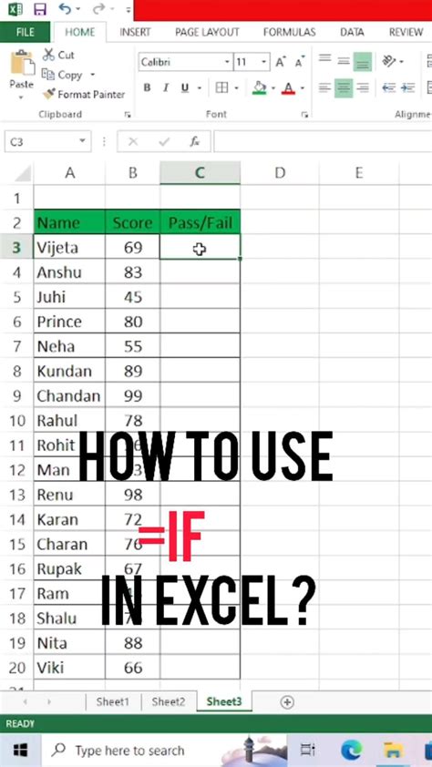
The IF function is one of the most commonly used formulas in Excel, and it's perfect for comparing cells. The syntax for the IF function is:
IF(logical_test, [value_if_true], [value_if_false])
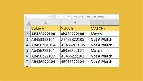
For example, suppose you want to compare two cells, A1 and B1. If the values are equal, you want to return "Match." Otherwise, you want to return "No Match."
=IF(A1=B1, "Match", "No Match")
Method 2: Using Conditional Formatting
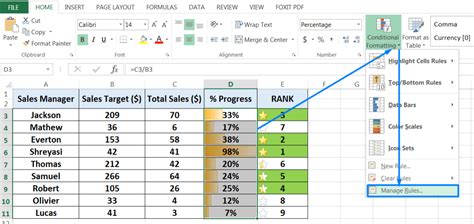
Conditional formatting is a powerful feature in Excel that allows you to highlight cells based on specific conditions. You can use conditional formatting to compare cells and highlight differences.
Select the cells you want to compare, go to the Home tab, and click on Conditional Formatting. Choose "New Rule" and then select "Use a formula to determine which cells to format."
= A1<>B1
This formula will highlight cells that are different.
Method 3: Using the EXACT Function
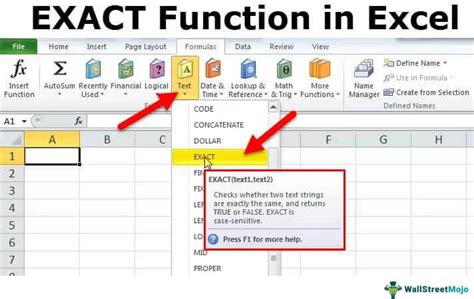
The EXACT function is a simple yet effective way to compare cells. The syntax for the EXACT function is:
EXACT(text1, text2)
For example, suppose you want to compare two cells, A1 and B1.
=EXACT(A1, B1)
This formula will return TRUE if the cells are identical and FALSE otherwise.
Method 4: Using the VLOOKUP Function
The VLOOKUP function is commonly used to search for values in a table, but you can also use it to compare cells. The syntax for the VLOOKUP function is:
VLOOKUP(lookup_value, table_array, col_index_num, [range_lookup])
For example, suppose you want to compare two cells, A1 and B1, and return a value from a third cell, C1.
=VLOOKUP(A1, B:C, 2, FALSE)
This formula will return the value in cell C1 if the value in cell A1 is found in column B.

Method 5: Using Power Query
Power Query is a powerful tool in Excel that allows you to manipulate and analyze data. You can use Power Query to compare cells by creating a new column with a formula.
Go to the Data tab, click on "From Table/Range," and select the table you want to compare. Then, go to the "Add Column" tab and click on "Custom Column."
=(A1 = B1)
This formula will create a new column with a value of TRUE or FALSE, indicating whether the cells are equal.

Conclusion
Comparing cells in Excel is a common task that can be achieved using various methods. Whether you're using formulas, conditional formatting, or Power Query, the key is to understand the basics of cell comparison and choose the method that best suits your needs. By mastering these techniques, you'll become more efficient and effective in your data analysis tasks.
Gallery of Excel Comparison Formulas
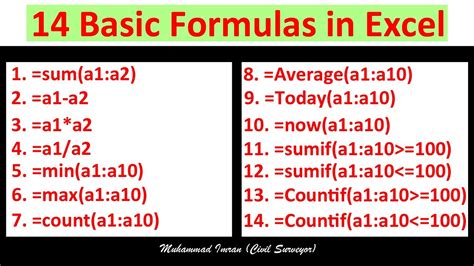
Excel Comparison Formulas

We hope this article has helped you learn new ways to compare cells in Excel. Do you have any favorite methods for comparing cells? Share your thoughts in the comments below!
