Excel Compare Two Lists For Duplicates Quickly

Comparing two lists in Excel for duplicates is a common task that can be time-consuming if done manually. However, with the right techniques and formulas, you can quickly and easily identify duplicate values between two lists.

Why Compare Two Lists for Duplicates?

Comparing two lists for duplicates is essential in various scenarios, such as:

• Data cleaning and validation: Identifying duplicate values helps ensure data accuracy and consistency.
• Data merging: Comparing lists helps prevent duplicate records when merging data from different sources.
• Data analysis: Duplicate values can affect data analysis results, so it's essential to identify and handle them properly.

Methods to Compare Two Lists for Duplicates

There are several methods to compare two lists for duplicates in Excel, including:

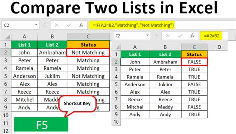
1. Using the IF Function: This method involves using the IF function to check if a value in one list exists in the other list.
2. Using the VLOOKUP Function: This method involves using the VLOOKUP function to search for values in one list within the other list.
3. Using Conditional Formatting: This method involves using conditional formatting to highlight duplicate values between two lists.
4. Using Power Query: This method involves using Power Query to compare two lists and identify duplicate values.

Method 1: Using the IF Function

To compare two lists using the IF function, follow these steps:

1. Select the cell where you want to display the result.
2. Type the formula: =IF(ISERROR(MATCH(A2, B:B, 0)), "Unique", "Duplicate")
3. Press Enter.
4. Drag the formula down to apply it to the rest of the cells.

Method 2: Using the VLOOKUP Function

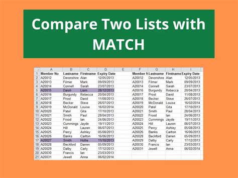
To compare two lists using the VLOOKUP function, follow these steps:

1. Select the cell where you want to display the result.
2. Type the formula: =IF(ISERROR(VLOOKUP(A2, B:B, 1, FALSE)), "Unique", "Duplicate")
3. Press Enter.
4. Drag the formula down to apply it to the rest of the cells.

Method 3: Using Conditional Formatting

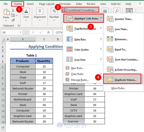
To compare two lists using conditional formatting, follow these steps:

1. Select the range of cells you want to format.
2. Go to the Home tab > Conditional Formatting > New Rule.
3. Select "Use a formula to determine which cells to format."
4. Type the formula: =COUNTIF(B:B, A2) > 0
5. Click Format and select a format.
6. Click OK.

Method 4: Using Power Query

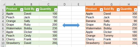
To compare two lists using Power Query, follow these steps:

1. Go to the Data tab > From Table/Range.
2. Select the range of cells you want to compare.
3. Click OK.
4. Go to the Home tab > Merge Queries.
5. Select the other list as the merge query.
6. Click OK.

Gallery of Excel Compare Two Lists

Excel Compare Two Lists Image Gallery

Conclusion

Comparing two lists in Excel for duplicates is a crucial task that can be accomplished using various methods. By using the IF function, VLOOKUP function, conditional formatting, or Power Query, you can quickly and easily identify duplicate values between two lists. Remember to choose the method that best suits your needs and data complexity.