Excel Conditional Formatting Based On Another Column

Excel conditional formatting is a powerful tool that allows you to highlight cells based on specific conditions, making it easier to analyze and understand your data. One of the most useful applications of conditional formatting is to format cells based on the values in another column. In this article, we will explore how to use Excel conditional formatting based on another column, including the benefits, steps, and examples.

Why Use Conditional Formatting Based on Another Column?

Conditional formatting based on another column is useful when you want to highlight cells in one column based on the values in another column. This can help you to:

• Identify trends and patterns in your data
• Highlight important information, such as errors or warnings
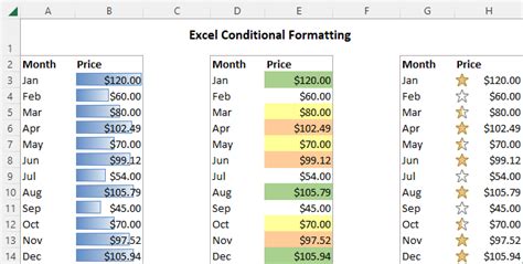
• Create visualizations that make it easier to understand complex data
• Automate formatting tasks, saving you time and reducing errors

How to Use Conditional Formatting Based on Another Column

To use conditional formatting based on another column, follow these steps:

1. Select the cells you want to format.
2. Go to the Home tab in the Excel ribbon.
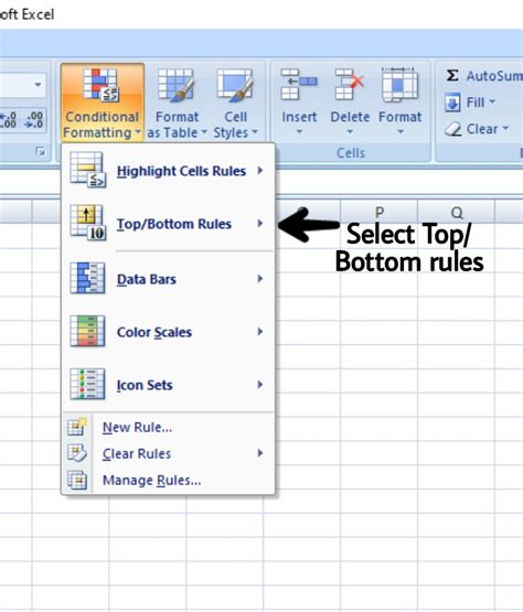
3. Click on the Conditional Formatting button in the Styles group.
4. Select "New Rule" from the drop-down menu.
5. Choose "Use a formula to determine which cells to format" from the list of options.
6. Enter a formula that references the column you want to base the formatting on. For example, if you want to format cells in column A based on the values in column B, you might enter the formula =B1>10.
7. Click on the Format button to select the formatting options you want to apply.
8. Click OK to apply the rule.

Examples of Conditional Formatting Based on Another Column

Here are a few examples of how you might use conditional formatting based on another column:

• Highlighting errors: Suppose you have a column of numbers that you want to check for errors. You can use conditional formatting to highlight any cells that contain errors, based on the values in another column. For example, you might enter the formula =ISERROR(B1) to highlight any cells in column A that contain errors in column B.
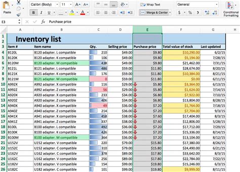
• Highlighting trends: Suppose you have a column of numbers that you want to analyze for trends. You can use conditional formatting to highlight any cells that are above or below a certain threshold, based on the values in another column. For example, you might enter the formula =B1>AVERAGE(B:B) to highlight any cells in column A that are above the average value in column B.
• Creating visualizations: Suppose you have a column of numbers that you want to visualize as a heatmap. You can use conditional formatting to format cells based on the values in another column, creating a heatmap that shows the distribution of values. For example, you might enter the formula =B1>10 to format cells in column A as green if the corresponding value in column B is greater than 10.

Common Formulas for Conditional Formatting Based on Another Column

Here are some common formulas you can use for conditional formatting based on another column:

• =B1>10 - Highlights cells in column A if the corresponding value in column B is greater than 10.
• =B1=AVERAGE(B:B) - Highlights cells in column A if the corresponding value in column B is equal to the average value in column B.
• =ISERROR(B1) - Highlights cells in column A if the corresponding value in column B contains an error.
• =B1>MAX(B:B) - Highlights cells in column A if the corresponding value in column B is greater than the maximum value in column B.

Tips and Tricks for Using Conditional Formatting Based on Another Column

Here are some tips and tricks for using conditional formatting based on another column:

• Use absolute references: When referencing cells in another column, use absolute references (e.g. $B$1) to ensure that the formula doesn't change when you copy and paste it.
• Use named ranges: If you have a large spreadsheet, it can be helpful to use named ranges to make it easier to reference cells in another column.
• Use multiple conditions: You can use multiple conditions in your formula to create more complex formatting rules. For example, you might enter the formula =AND(B1>10, C1<20) to highlight cells in column A if the corresponding value in column B is greater than 10 and the corresponding value in column C is less than 20.

Common Errors to Avoid When Using Conditional Formatting Based on Another Column

Here are some common errors to avoid when using conditional formatting based on another column:

• Incorrect references: Make sure to use the correct references when referencing cells in another column. If you use relative references (e.g. B1), the formula may not work correctly when you copy and paste it.
• Typos in formulas: Typos in formulas can cause errors and prevent the formatting from working correctly. Make sure to double-check your formulas for typos and syntax errors.
• Overlapping formatting rules: If you have multiple formatting rules that overlap, it can cause errors and prevent the formatting from working correctly. Make sure to check for overlapping rules and adjust them as needed.

Gallery of Excel Conditional Formatting Examples

Excel Conditional Formatting Image Gallery

Conclusion

Excel conditional formatting based on another column is a powerful tool that can help you to analyze and understand your data more effectively. By using formulas and formatting rules, you can create visualizations that highlight trends and patterns in your data, making it easier to identify important information and make informed decisions. With the tips and tricks outlined in this article, you can use conditional formatting based on another column to take your data analysis to the next level.

We hope this article has been helpful in explaining how to use Excel conditional formatting based on another column. If you have any questions or need further assistance, please don't hesitate to ask.