5 Ways To Apply Excel Conditional Formatting For Text

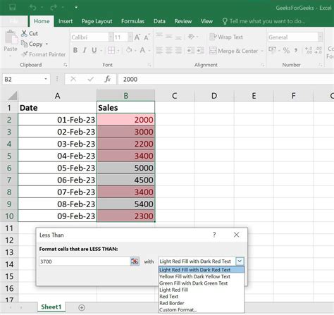
Excel is a powerful tool that allows users to manage and analyze large datasets with ease. One of its most useful features is conditional formatting, which enables users to highlight cells based on specific conditions. In this article, we will explore five ways to apply Excel conditional formatting for text, making it easier to identify trends, patterns, and outliers in your data.

Why Use Conditional Formatting for Text?

Conditional formatting is a game-changer when it comes to data analysis. By highlighting cells based on specific conditions, you can quickly identify trends, patterns, and outliers in your data. This feature is particularly useful when working with large datasets, as it allows you to visualize your data and make informed decisions. In the context of text data, conditional formatting can help you identify specific keywords, phrases, or patterns, making it easier to analyze and understand your data.

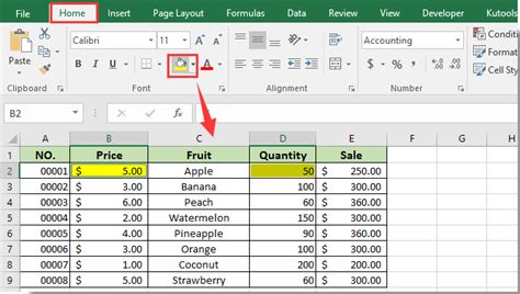
Method 1: Highlighting Cells with Specific Text

One of the most common uses of conditional formatting for text is to highlight cells that contain specific text. To do this, follow these steps:

1. Select the range of cells you want to format.
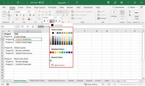
2. Go to the Home tab in the Excel ribbon.
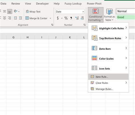
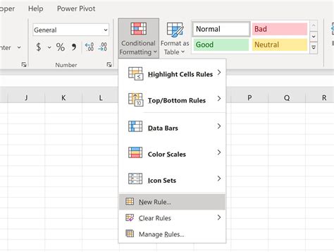
3. Click on the Conditional Formatting button in the Styles group.
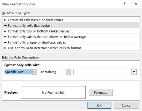
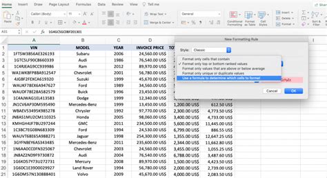
4. Select "New Rule" from the drop-down menu.
5. Choose "Use a formula to determine which cells to format" from the list of options.
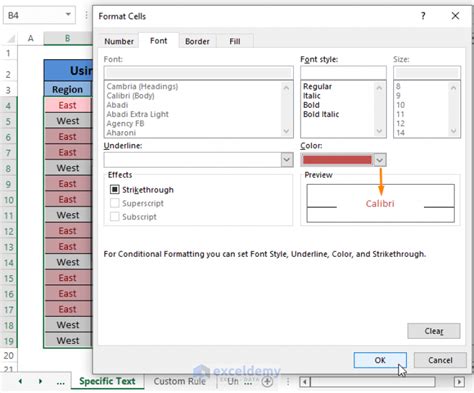
6. Enter the formula =A1="specific text" (replace "specific text" with the text you want to highlight).
7. Click on the Format button and select the desired formatting options.
8. Click OK to apply the rule.

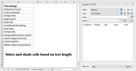
Method 2: Highlighting Cells with Text Length

Another useful application of conditional formatting for text is to highlight cells based on the length of the text. For example, you may want to highlight cells that contain text that is longer than a certain number of characters. To do this, follow these steps:

1. Select the range of cells you want to format.
2. Go to the Home tab in the Excel ribbon.
3. Click on the Conditional Formatting button in the Styles group.
4. Select "New Rule" from the drop-down menu.
5. Choose "Use a formula to determine which cells to format" from the list of options.
6. Enter the formula =LEN(A1)>10 (replace 10 with the desired text length).
7. Click on the Format button and select the desired formatting options.
8. Click OK to apply the rule.

Method 3: Highlighting Cells with Text Containing Numbers

If you want to highlight cells that contain text with numbers, you can use the following method:

1. Select the range of cells you want to format.
2. Go to the Home tab in the Excel ribbon.
3. Click on the Conditional Formatting button in the Styles group.
4. Select "New Rule" from the drop-down menu.
5. Choose "Use a formula to determine which cells to format" from the list of options.
6. Enter the formula =ISNUMBER(SUBSTITUTE(A1," ","")) (this formula removes spaces and checks if the resulting text is a number).
7. Click on the Format button and select the desired formatting options.
8. Click OK to apply the rule.

Method 4: Highlighting Cells with Text Containing Specific Phrases

If you want to highlight cells that contain specific phrases, you can use the following method:

1. Select the range of cells you want to format.
2. Go to the Home tab in the Excel ribbon.
3. Click on the Conditional Formatting button in the Styles group.
4. Select "New Rule" from the drop-down menu.
5. Choose "Use a formula to determine which cells to format" from the list of options.
6. Enter the formula =SEARCH("specific phrase",A1)>0 (replace "specific phrase" with the phrase you want to highlight).
7. Click on the Format button and select the desired formatting options.
8. Click OK to apply the rule.

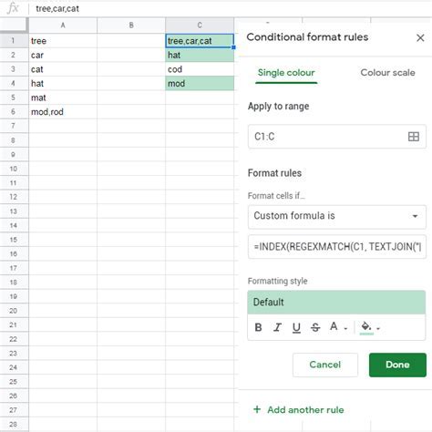
Method 5: Highlighting Cells with Text Using Regular Expressions

If you want to highlight cells that contain text that matches a specific pattern, you can use regular expressions. To do this, follow these steps:

1. Select the range of cells you want to format.
2. Go to the Home tab in the Excel ribbon.
3. Click on the Conditional Formatting button in the Styles group.
4. Select "New Rule" from the drop-down menu.
5. Choose "Use a formula to determine which cells to format" from the list of options.
6. Enter the formula =REGEX(A1,"pattern") (replace "pattern" with the regular expression you want to use).
7. Click on the Format button and select the desired formatting options.
8. Click OK to apply the rule.

Gallery of Conditional Formatting for Text

Conditional Formatting for Text Image Gallery

Conclusion

Conditional formatting is a powerful feature in Excel that allows you to highlight cells based on specific conditions. In this article, we explored five ways to apply Excel conditional formatting for text, including highlighting cells with specific text, text length, text containing numbers, text containing specific phrases, and text using regular expressions. By mastering these techniques, you can take your data analysis to the next level and make informed decisions.

Take Action

Now that you've learned about the different ways to apply Excel conditional formatting for text, it's time to put your skills into practice. Try out these techniques on your own dataset and see how they can help you gain insights and make informed decisions. If you have any questions or need further assistance, feel free to comment below.