Excel Conditional Formatting With Text Contains Formula

Excel's conditional formatting feature is a powerful tool that allows you to highlight cells based on specific conditions. One of the most useful formulas in conditional formatting is the "Text Contains" formula, which enables you to format cells based on the presence of specific text within a cell.

The "Text Contains" formula is a great way to quickly identify cells that contain specific keywords or phrases, making it easier to analyze and visualize your data. In this article, we will explore how to use the "Text Contains" formula in Excel's conditional formatting feature.

Why Use Conditional Formatting?

Conditional formatting is a powerful feature in Excel that allows you to format cells based on specific conditions. This feature can help you to:

• Highlight important information
• Identify trends and patterns
• Create visualizations to aid in data analysis
• Simplify complex data sets

Using the "Text Contains" Formula

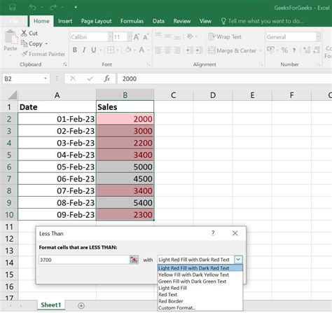
To use the "Text Contains" formula in Excel's conditional formatting feature, follow these steps:

1. Select the range of cells that you want to format.
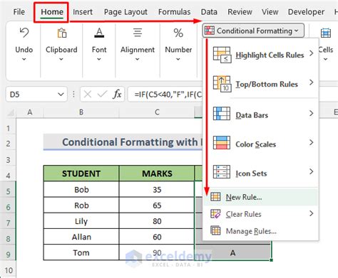
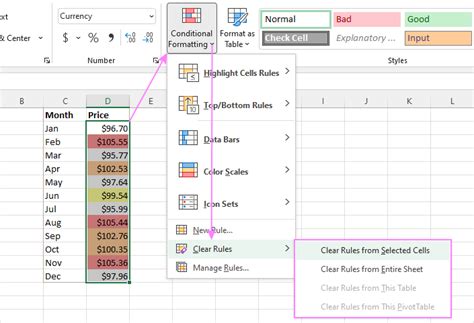
2. Go to the "Home" tab in the Excel ribbon.
3. Click on the "Conditional Formatting" button in the "Styles" group.
4. Select "New Rule" from the drop-down menu.
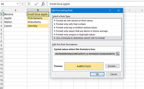
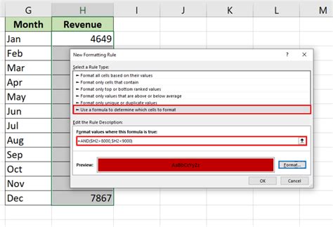
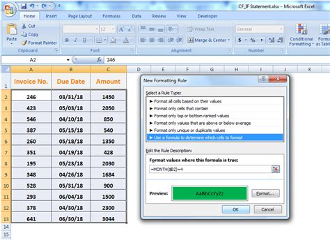
5. Choose "Use a formula to determine which cells to format".
6. In the formula bar, enter the following formula: =ISNUMBER(SEARCH("keyword",A1))

Replace "keyword" with the text that you want to search for, and A1 with the cell that you want to search.

7. Click on the "Format" button to select the formatting options.
8. Click on the "OK" button to apply the formatting.

The formula =ISNUMBER(SEARCH("keyword",A1)) uses the SEARCH function to search for the specified text within the cell. The ISNUMBER function then checks if the result of the SEARCH function is a number, indicating that the text was found.

Example

Suppose you have a list of products in column A, and you want to highlight cells that contain the word "electronic". You can use the following formula: =ISNUMBER(SEARCH("electronic",A1))

Tips and Variations

• To search for multiple keywords, use the OR function: =OR(ISNUMBER(SEARCH("keyword1",A1)),ISNUMBER(SEARCH("keyword2",A1)))
• To search for a phrase, use the SEARCH function with the phrase enclosed in quotes: =ISNUMBER(SEARCH("electronic devices",A1))
• To search for a word that starts with a specific letter, use the LEFT function: =ISNUMBER(SEARCH("e*",A1))
• To search for a word that ends with a specific letter, use the RIGHT function: =ISNUMBER(SEARCH("*e",A1))

Gallery of Excel Conditional Formatting Examples

Excel Conditional Formatting Examples

Conclusion

In this article, we explored the "Text Contains" formula in Excel's conditional formatting feature. We demonstrated how to use this formula to highlight cells that contain specific text, and provided tips and variations for more advanced searches. By using this formula, you can simplify complex data sets and create visualizations to aid in data analysis.

We hope this article has been helpful in improving your Excel skills. If you have any questions or comments, please feel free to share them with us.