5 Ways To Filter Excel Rows Instead Of Columns

In Microsoft Excel, filtering data is a crucial step in analyzing and understanding large datasets. While most users are familiar with filtering columns, there are scenarios where filtering rows is necessary. In this article, we will explore five ways to filter Excel rows instead of columns.

Understanding the Need for Row Filtering

Before we dive into the methods, it's essential to understand why row filtering is necessary. In a typical Excel spreadsheet, columns represent categories or fields, while rows represent individual data points or records. However, there are situations where you might want to filter rows based on specific conditions, such as:

Identifying duplicates or unique values across multiple columns
Filtering data based on a specific pattern or format
Hiding or showing rows that meet certain criteria

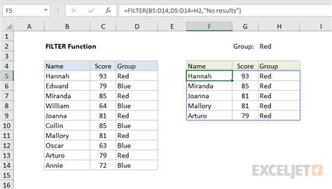
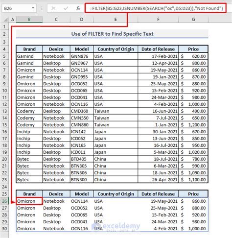
Method 1: Using the FILTER Function

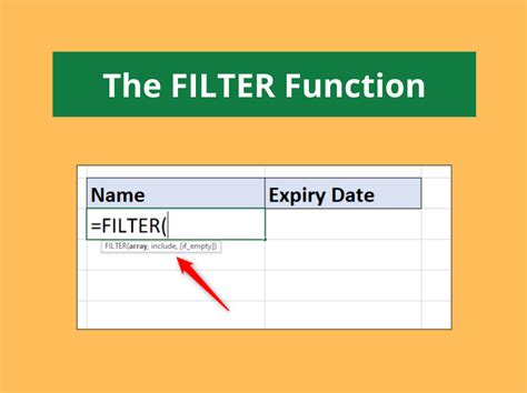
One of the most straightforward ways to filter rows in Excel is by using the FILTER function, introduced in Excel 2019 and later versions. The FILTER function allows you to filter an array or range based on a specific condition.

The syntax for the FILTER function is:

FILTER(array, include, [if_empty])

Where:

array is the range or array you want to filter
include is the condition that determines which rows to include
[if_empty] is the value to return if the filtered array is empty

For example, to filter rows where the value in column A is greater than 10, you can use the following formula:

=FILTER(A1:C10, A1:A10 > 10)

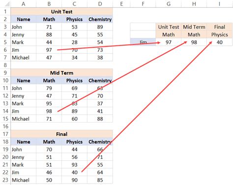
Method 2: Using the INDEX and MATCH Functions

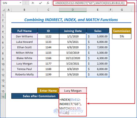
Using the INDEX and MATCH functions in Excel

Another way to filter rows in Excel is by using the INDEX and MATCH functions. This method involves creating a helper column that contains a formula that returns a row number if the condition is met.

The syntax for the INDEX and MATCH functions is:

=INDEX(range, MATCH(lookup_value, lookup_array, [match_type])

Where:

range is the range or array you want to filter
lookup_value is the value you want to look up
lookup_array is the range or array that contains the values to look up
[match_type] is the type of match ( exact or approximate)

For example, to filter rows where the value in column A is greater than 10, you can use the following formula:

=INDEX(A1:C10, MATCH(1, (A1:A10 > 10), 0))

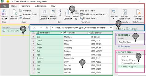
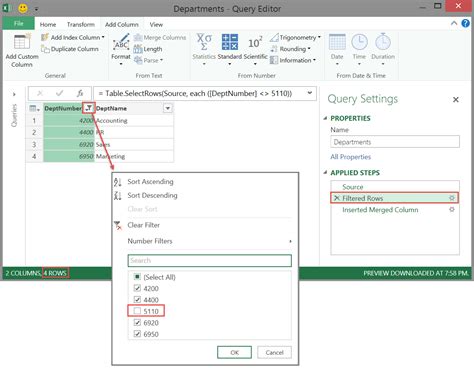
Method 3: Using Power Query

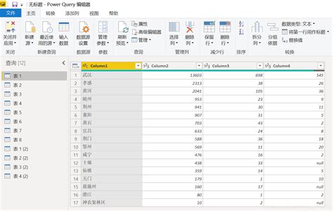
Power Query is a powerful data manipulation tool in Excel that allows you to filter rows based on specific conditions. To use Power Query, you need to create a new query and then filter the data using the Filter function.

To filter rows in Power Query, follow these steps:

Go to the Data tab and click on New Query
Select the range or table you want to filter
Go to the Home tab and click on Filter
Select the condition you want to apply

For example, to filter rows where the value in column A is greater than 10, you can use the following formula:

= Table.SelectRows(#"Previous Step", each [Column A] > 10)

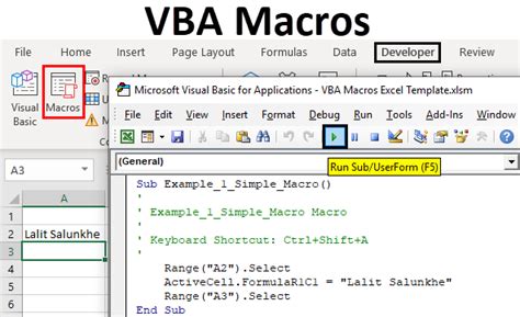
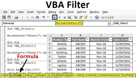
Method 4: Using VBA Macros

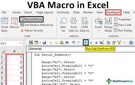
VBA macros are a powerful way to automate tasks in Excel, including filtering rows. To filter rows using VBA macros, you need to create a new module and then write a script that filters the data based on a specific condition.

For example, to filter rows where the value in column A is greater than 10, you can use the following script:

Sub FilterRows() Dim ws As Worksheet Set ws = ThisWorkbook.Worksheets("Sheet1") Dim lastRow As Long lastRow = ws.Cells(ws.Rows.Count, "A").End(xlUp).Row For i = 1 To lastRow If ws.Cells(i, 1).Value > 10 Then ws.Rows(i).Hidden = False Else ws.Rows(i).Hidden = True End If Next i End Sub

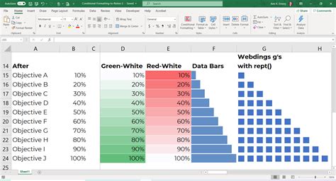
Method 5: Using Conditional Formatting

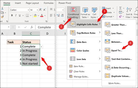
Conditional formatting is a feature in Excel that allows you to highlight cells based on specific conditions. While it's not a traditional filtering method, you can use conditional formatting to filter rows by highlighting the rows that meet a specific condition.

To filter rows using conditional formatting, follow these steps:

Select the range or table you want to filter
Go to the Home tab and click on Conditional Formatting
Select New Rule
Select the condition you want to apply

For example, to filter rows where the value in column A is greater than 10, you can use the following formula:

=A1>10

Conclusion

Filtering rows in Excel can be a bit tricky, but with the right techniques, you can achieve the desired results. In this article, we explored five ways to filter Excel rows instead of columns, including using the FILTER function, INDEX and MATCH functions, Power Query, VBA macros, and conditional formatting. By mastering these techniques, you can take your data analysis skills to the next level.

Gallery of Row Filtering Techniques

Row Filtering Techniques Image Gallery

Filter rows based on multiple conditions

We hope this article has been helpful in teaching you how to filter rows in Excel. If you have any questions or need further assistance, please don't hesitate to ask.