5 Ways To Find Duplicates In Multiple Excel Columns

In the world of data analysis, duplicates can be a major headache. When working with multiple Excel columns, finding duplicates can be a daunting task, especially if you're dealing with a large dataset. But fear not, dear Excel enthusiasts! We've got five effective ways to help you find duplicates in multiple Excel columns.

Understanding the Importance of Finding Duplicates

Before we dive into the methods, let's quickly discuss why finding duplicates is crucial. Duplicates can lead to inaccurate analysis, skewed results, and poor decision-making. By identifying and removing duplicates, you can ensure the integrity of your data and make informed decisions.

Method 1: Using Conditional Formatting

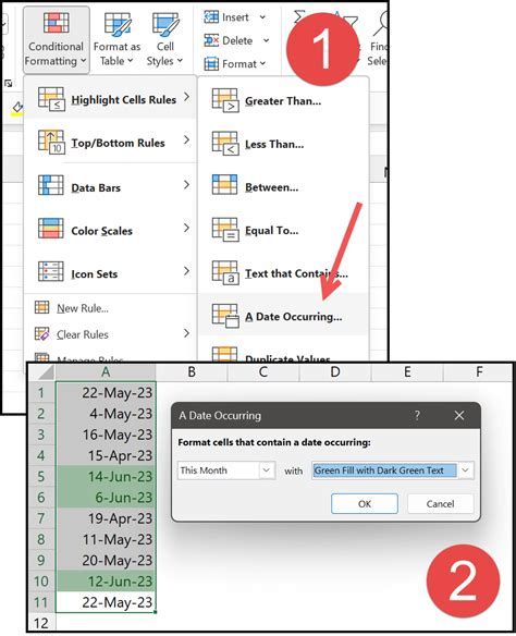
Conditional formatting is a powerful feature in Excel that allows you to highlight duplicates based on specific conditions. To use this method:

Select the columns you want to check for duplicates.
Go to the "Home" tab > "Styles" > "Conditional Formatting" > "New Rule".
Choose "Use a formula to determine which cells to format".
Enter the formula: =COUNTIFS(A:A, A2, B:B, B2)>1 (assuming your data is in columns A and B).
Format the cells as desired (e.g., highlight them in yellow).

This method will highlight duplicate values in both columns.

Method 2: Using the VLOOKUP Function

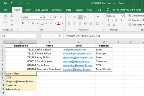
The VLOOKUP function is another powerful tool in Excel that can help you find duplicates. To use this method:

Select a cell where you want to display the duplicate values.
Enter the formula: =VLOOKUP(A2, B:C, 2, FALSE) (assuming your data is in columns A and B).
If the value is found, the formula will return the value; otherwise, it will return a #N/A error.
Use the IFERROR function to display a message when no duplicates are found: =IFERROR(VLOOKUP(A2, B:C, 2, FALSE), "No duplicates found").

This method will return the duplicate values in column B.

Method 3: Using the FILTER Function

The FILTER function is a new addition to Excel that allows you to filter data based on specific conditions. To use this method:

Select a cell where you want to display the duplicate values.
Enter the formula: =FILTER(A:B, COUNTIFS(A:A, A:A, B:B, B:B)>1) (assuming your data is in columns A and B).
The formula will return the duplicate values in both columns.

This method is similar to the conditional formatting method but returns the duplicate values instead of highlighting them.

Method 4: Using the Remove Duplicates Feature

Excel's Remove Duplicates feature is a quick and easy way to find duplicates. To use this method:

Select the columns you want to check for duplicates.
Go to the "Data" tab > "Data Tools" > "Remove Duplicates".
Choose the columns you want to check for duplicates.
Click "OK".

This method will remove duplicates from the selected columns.

Method 5: Using Power Query

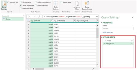
Power Query is a powerful tool in Excel that allows you to manipulate and analyze data. To use this method:

Select the columns you want to check for duplicates.
Go to the "Data" tab > "Get & Transform Data" > "From Table/Range".
Create a new query.
Use the Group By feature to group the data by the columns you want to check for duplicates.
Use the Count feature to count the number of duplicates.
Load the query into a new worksheet.

This method will return the duplicate values in a new worksheet.

Gallery of Duplicate Detection Methods

Duplicate Detection Methods

In conclusion, finding duplicates in multiple Excel columns can be a challenging task, but with the right techniques, it can be done efficiently. Whether you use conditional formatting, the VLOOKUP function, the FILTER function, the Remove Duplicates feature, or Power Query, you'll be able to identify and remove duplicates from your data.