
Unlocking the Power of VLOOKUP in Excel for Mac
VLOOKUP is one of the most powerful and versatile functions in Excel, allowing users to search for specific data in a table and return corresponding values. As a Mac user, you can harness the full potential of VLOOKUP in Excel to streamline your workflow, simplify complex tasks, and make data analysis more efficient. In this article, we'll explore seven essential VLOOKUP formulas that every Excel user on Mac should know.
Why VLOOKUP is Essential in Excel
Before diving into the formulas, let's quickly discuss why VLOOKUP is a game-changer in Excel. VLOOKUP enables you to:
- Search for specific data in a table or range
- Return corresponding values from another column
- Simplify data analysis and reduce errors
- Improve productivity and workflow efficiency
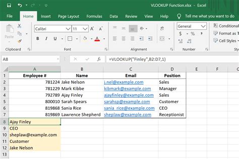
Formula 1: Basic VLOOKUP Syntax
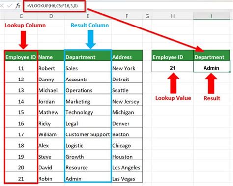
The basic VLOOKUP syntax is:
VLOOKUP(lookup_value, table_array, col_index_num, [range_lookup])
lookup_value: the value you want to search fortable_array: the range of cells containing the datacol_index_num: the column number containing the value you want to return[range_lookup]: optional, specify TRUE for approximate match or FALSE for exact match
Example:
Suppose you have a table with employee names, departments, and salaries, and you want to find the salary of a specific employee. You can use the VLOOKUP formula like this:
=VLOOKUP("John Doe", A2:C10, 3, FALSE)
This formula searches for "John Doe" in the first column of the table, returns the corresponding value in the third column (salary), and specifies an exact match.
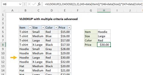
Formula 2: Using VLOOKUP with Multiple Criteria
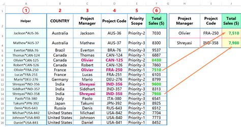
When you need to search for data based on multiple criteria, you can use the VLOOKUP function in combination with the INDEX and MATCH functions.
=INDEX(C:C, MATCH(1, (A:A = "John Doe") * (B:B = "Sales"), 0))
INDEX(C:C, MATCH(1, (A:A = "John Doe") * (B:B = "Sales"), 0)): returns the value in column C where the conditions are met
Example:
Suppose you have a table with employee names, departments, and sales data, and you want to find the sales data for a specific employee in a specific department. You can use the VLOOKUP formula like this:
=INDEX(C:C, MATCH(1, (A:A = "John Doe") * (B:B = "Sales"), 0))
This formula searches for "John Doe" in the first column and "Sales" in the second column, returns the corresponding value in column C (sales data), and specifies an exact match.
Formula 3: Using VLOOKUP with Multiple Tables
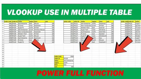
When you need to search for data in multiple tables, you can use the VLOOKUP function in combination with the CHOOSE function.
=CHOOSE(MATCH("John Doe", A:A, 0), VLOOKUP("John Doe", A2:C10, 3, FALSE), VLOOKUP("John Doe", E2:G10, 3, FALSE))
CHOOSE(MATCH("John Doe", A:A, 0), VLOOKUP("John Doe", A2:C10, 3, FALSE), VLOOKUP("John Doe", E2:G10, 3, FALSE)): returns the value from either table based on the match
Example:
Suppose you have two tables with employee names, departments, and salaries, and you want to find the salary of a specific employee. You can use the VLOOKUP formula like this:
=CHOOSE(MATCH("John Doe", A:A, 0), VLOOKUP("John Doe", A2:C10, 3, FALSE), VLOOKUP("John Doe", E2:G10, 3, FALSE))
This formula searches for "John Doe" in the first column of either table, returns the corresponding value in the third column (salary), and specifies an exact match.
Formula 4: Using VLOOKUP with Dynamic Ranges
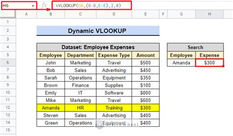
When you need to search for data in a dynamic range, you can use the VLOOKUP function in combination with the OFFSET and MATCH functions.
=VLOOKUP("John Doe", OFFSET(A1, 0, 0, MATCH("John Doe", A:A, 0), 3), 3, FALSE)
OFFSET(A1, 0, 0, MATCH("John Doe", A:A, 0), 3): returns the range of cells based on the match
Example:
Suppose you have a table with employee names, departments, and salaries, and you want to find the salary of a specific employee. You can use the VLOOKUP formula like this:
=VLOOKUP("John Doe", OFFSET(A1, 0, 0, MATCH("John Doe", A:A, 0), 3), 3, FALSE)
This formula searches for "John Doe" in the first column, returns the corresponding value in the third column (salary), and specifies an exact match.
Formula 5: Using VLOOKUP with Dates
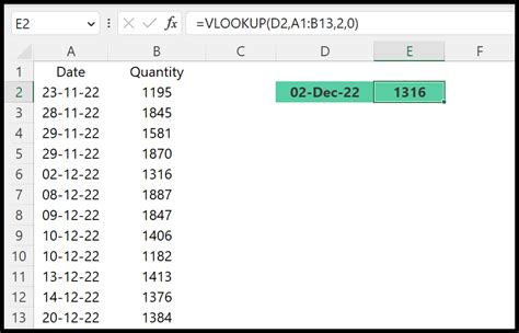
When you need to search for data based on dates, you can use the VLOOKUP function in combination with the DATE and MATCH functions.
=VLOOKUP(DATE(2022, 1, 1), A2:C10, 3, FALSE)
DATE(2022, 1, 1): returns the date in the format YYYY-MM-DD
Example:
Suppose you have a table with dates, sales data, and employee names, and you want to find the sales data for a specific date. You can use the VLOOKUP formula like this:
=VLOOKUP(DATE(2022, 1, 1), A2:C10, 3, FALSE)
This formula searches for the date in the first column, returns the corresponding value in the third column (sales data), and specifies an exact match.
Formula 6: Using VLOOKUP with Errors
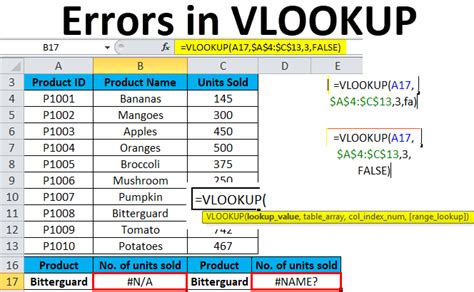
When you need to handle errors in your VLOOKUP formula, you can use the IFERROR function.
=IFERROR(VLOOKUP("John Doe", A2:C10, 3, FALSE), "Not Found")
IFERROR(VLOOKUP("John Doe", A2:C10, 3, FALSE), "Not Found"): returns the value if found, otherwise returns "Not Found"
Example:
Suppose you have a table with employee names, departments, and salaries, and you want to find the salary of a specific employee. You can use the VLOOKUP formula like this:
=IFERROR(VLOOKUP("John Doe", A2:C10, 3, FALSE), "Not Found")
This formula searches for "John Doe" in the first column, returns the corresponding value in the third column (salary), and specifies an exact match. If the value is not found, it returns "Not Found".
Formula 7: Using VLOOKUP with Multiple Lookups
When you need to perform multiple lookups in your VLOOKUP formula, you can use the CHOOSE and MATCH functions.
=CHOOSE(MATCH("John Doe", A:A, 0), VLOOKUP("John Doe", A2:C10, 3, FALSE), VLOOKUP("John Doe", E2:G10, 3, FALSE))
CHOOSE(MATCH("John Doe", A:A, 0), VLOOKUP("John Doe", A2:C10, 3, FALSE), VLOOKUP("John Doe", E2:G10, 3, FALSE)): returns the value from either table based on the match
Example:
Suppose you have two tables with employee names, departments, and salaries, and you want to find the salary of a specific employee. You can use the VLOOKUP formula like this:
=CHOOSE(MATCH("John Doe", A:A, 0), VLOOKUP("John Doe", A2:C10, 3, FALSE), VLOOKUP("John Doe", E2:G10, 3, FALSE))
This formula searches for "John Doe" in the first column of either table, returns the corresponding value in the third column (salary), and specifies an exact match.
VLOOKUP Formulas for Excel on Mac Gallery


We hope this article has helped you unlock the full potential of VLOOKUP in Excel for Mac. With these seven essential formulas, you can simplify complex tasks, improve productivity, and make data analysis more efficient. Remember to experiment with different formulas and combinations to achieve the desired results. If you have any questions or need further assistance, feel free to ask in the comments below.