Display Excel Pivot Table Values As Text Easily

Excel pivot tables are a powerful tool for data analysis, allowing users to summarize and analyze large datasets with ease. One common requirement when working with pivot tables is to display values as text, rather than numbers. In this article, we will explore the different ways to display Excel pivot table values as text, and provide tips and tricks to make the process easier.

Why Display Pivot Table Values as Text?

There are several reasons why you might want to display pivot table values as text. For example:

• To display categorical data, such as product names or regions, which are not numerical in nature.
• To show text-based metrics, such as survey responses or customer feedback.
• To create a more readable and user-friendly report, by displaying text summaries instead of numerical values.

Method 1: Using the "Value Field Settings" Option

One way to display pivot table values as text is to use the "Value Field Settings" option. To do this:

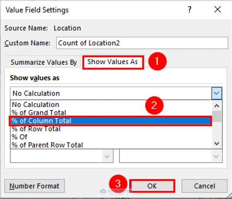
1. Select the pivot table cell that contains the value you want to display as text.
2. Right-click on the cell and select "Value Field Settings".
3. In the "Value Field Settings" dialog box, click on the "Number Format" button.
4. Select "Text" from the list of available formats.
5. Click "OK" to apply the changes.

Method 2: Using the "Text" Function

Another way to display pivot table values as text is to use the "Text" function. To do this:

1. Select the pivot table cell that contains the value you want to display as text.
2. Type the following formula: =TEXT(A1,""), where A1 is the cell that contains the value.
3. Press Enter to apply the formula.

Method 3: Using Conditional Formatting

You can also use conditional formatting to display pivot table values as text. To do this:

1. Select the pivot table cell that contains the value you want to display as text.
2. Go to the "Home" tab in the Excel ribbon.
3. Click on the "Conditional Formatting" button.
4. Select "New Rule".
5. In the "Format values where this formula is true" field, enter the following formula: =ISTEXT(A1), where A1 is the cell that contains the value.
6. Click "OK" to apply the rule.

Tips and Tricks

Here are some tips and tricks to help you display pivot table values as text more easily:

• Use the "Text" function to display text values, as it is more flexible and powerful than the "Value Field Settings" option.
• Use conditional formatting to highlight text values, and make your pivot table more readable.
• Use the "ISTEXT" function to check if a value is text, and apply formatting accordingly.
• Use the "IF" function to apply different formatting rules based on the value type.

Gallery of Pivot Table Text Display Options

Pivot Table Text Display Options

Frequently Asked Questions

Q: How do I display pivot table values as text in Excel? A: You can display pivot table values as text using the "Value Field Settings" option, the "Text" function, or conditional formatting.

Q: What is the difference between the "Value Field Settings" option and the "Text" function? A: The "Value Field Settings" option is a built-in feature in Excel that allows you to format values as text, while the "Text" function is a more flexible and powerful way to display text values.

Q: Can I use conditional formatting to display pivot table values as text? A: Yes, you can use conditional formatting to highlight text values and make your pivot table more readable.

Conclusion

In this article, we have explored the different ways to display Excel pivot table values as text, and provided tips and tricks to make the process easier. Whether you use the "Value Field Settings" option, the "Text" function, or conditional formatting, displaying pivot table values as text can help you create more readable and user-friendly reports.