
Finding Entire Rows in Excel: A Comprehensive Guide

When working with large datasets in Excel, it's not uncommon to need to find and return entire rows based on specific criteria. Whether you're looking for a particular value, a range of values, or even a specific format, Excel provides several ways to achieve this. In this article, we'll explore five methods to return entire rows in Excel if a match is found.
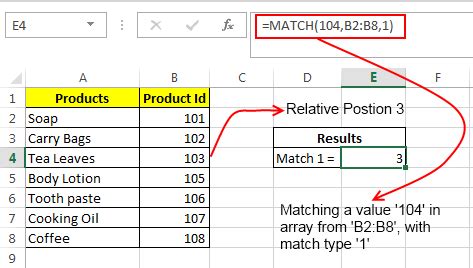
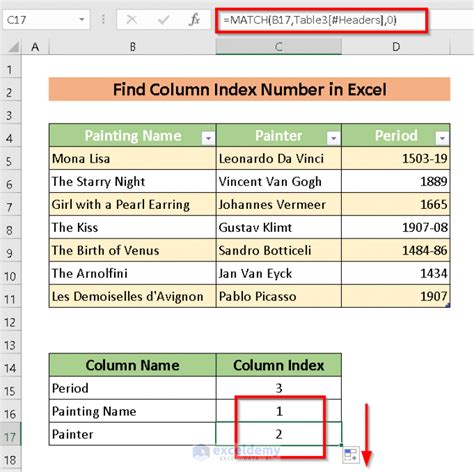
Method 1: Using the INDEX-MATCH Function Combination
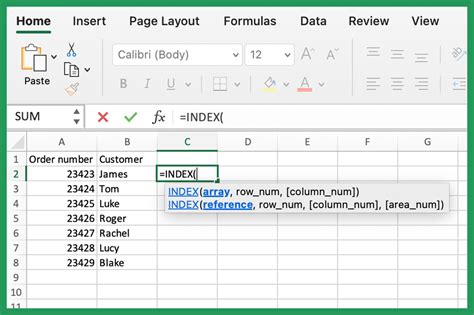
One of the most popular and powerful methods to return entire rows in Excel is by using the INDEX-MATCH function combination. This method is particularly useful when you need to search for a value in a specific column and return the corresponding row.
The syntax for this formula is:
INDEX(range, MATCH(lookup_value, lookup_array, [match_type])
Where:
rangeis the range of cells that you want to returnlookup_valueis the value that you want to search forlookup_arrayis the range of cells that you want to search in[match_type]is the type of match that you want to perform (optional)
For example, suppose you have a dataset in the range A1:E10, and you want to find the entire row where the value in column A is "John". You can use the following formula:
INDEX(A:E, MATCH("John", A:A, 0))
This formula will return the entire row where the value in column A is "John".
Method 2: Using the FILTER Function
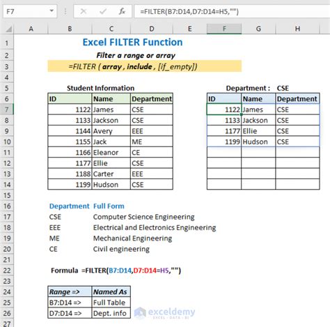
Another method to return entire rows in Excel is by using the FILTER function. This function is available in Excel 2019 and later versions.
The syntax for this formula is:
FILTER(range, criteria)
Where:
rangeis the range of cells that you want to returncriteriais the criteria that you want to apply to the range
For example, suppose you have a dataset in the range A1:E10, and you want to find the entire row where the value in column A is "John". You can use the following formula:
FILTER(A:E, A:A = "John")
This formula will return the entire row where the value in column A is "John".
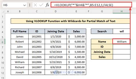
Method 3: Using the VLOOKUP Function
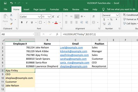
The VLOOKUP function is another popular method to return entire rows in Excel. However, this method has some limitations, as it can only return values from a single column.
The syntax for this formula is:
VLOOKUP(lookup_value, table_array, col_index_num, [range_lookup])
Where:
lookup_valueis the value that you want to search fortable_arrayis the range of cells that you want to search incol_index_numis the column index number that you want to return[range_lookup]is the type of match that you want to perform (optional)
For example, suppose you have a dataset in the range A1:E10, and you want to find the value in column B where the value in column A is "John". You can use the following formula:
VLOOKUP("John", A:B, 2, FALSE)
This formula will return the value in column B where the value in column A is "John".
Method 4: Using the POWER QUERY Function
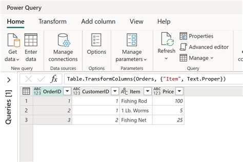
The POWER QUERY function is a powerful method to return entire rows in Excel. This function is available in Excel 2010 and later versions.
The syntax for this formula is:
=TABLEisselection
Where:
TABLEis the table that you want to queryisselectionis the selection that you want to apply to the table
For example, suppose you have a dataset in the range A1:E10, and you want to find the entire row where the value in column A is "John". You can use the following formula:
=TABLEisselection(#"Filtered Table", [Column1] = "John")
This formula will return the entire row where the value in column A is "John".
Method 5: Using the XLOOKUP Function
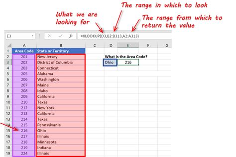
The XLOOKUP function is a new function in Excel that replaces the VLOOKUP function. This function is available in Excel 2019 and later versions.
The syntax for this formula is:
XLOOKUP(lookup_value, table_array, col_index_num, [if_not_found], [match_mode], [search_mode])
Where:
lookup_valueis the value that you want to search fortable_arrayis the range of cells that you want to search incol_index_numis the column index number that you want to return[if_not_found]is the value that you want to return if the lookup value is not found[match_mode]is the type of match that you want to perform (optional)[search_mode]is the search mode that you want to use (optional)
For example, suppose you have a dataset in the range A1:E10, and you want to find the value in column B where the value in column A is "John". You can use the following formula:
XLOOKUP("John", A:B, 2, "Not Found", FALSE, FALSE)
This formula will return the value in column B where the value in column A is "John".
Gallery of Excel Match Images
Excel Match Image Gallery


We hope this article has helped you to understand the different methods to return entire rows in Excel if a match is found. Whether you're using the INDEX-MATCH function combination, the FILTER function, the VLOOKUP function, the POWER QUERY function, or the XLOOKUP function, each method has its own strengths and weaknesses. By choosing the right method for your specific needs, you can simplify your workflow and become more efficient in your data analysis tasks.