Using multiple columns with the SUMIFS function in Excel can significantly enhance your data analysis capabilities. The SUMIFS function allows you to sum values in a specific column based on multiple conditions applied to different columns. This functionality is particularly useful in scenarios where you need to analyze data based on various criteria.
In this article, we will explore five ways to use the SUMIFS function with multiple columns in Excel, providing practical examples and explanations to help you master this powerful tool.

What is the SUMIFS Function?
The SUMIFS function is a multiple criteria summing function in Excel, which allows you to sum values in a specific column based on multiple conditions applied to different columns. The general syntax of the SUMIFS function is as follows:
SUMIFS(sum_range, criteria_range1, criteria1, [criteria_range2], [criteria2],...)
Where:
sum_rangeis the range of cells that you want to sum.criteria_range1is the first range of cells that you want to apply the criteria to.criteria1is the first criteria that you want to apply.[criteria_range2]and[criteria2]are optional and represent the second range of cells and criteria to apply.
1. Basic Usage of SUMIFS with Multiple Columns
Let's start with a basic example. Suppose we have a table with the following columns: Region, Product, Sales. We want to sum the sales for the North region and Product A.
| Region | Product | Sales |
|---|---|---|
| North | Product A | 100 |
| North | Product B | 200 |
| South | Product A | 300 |
| South | Product B | 400 |
Using the SUMIFS function, we can achieve this as follows:
=SUMIFS(C:C, A:A, "North", B:B, "Product A")
This formula sums the values in column C (Sales) where the value in column A (Region) is North and the value in column B (Product) is Product A.

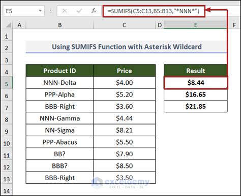
2. Using SUMIFS with Multiple Columns and Wildcards
Suppose we want to sum the sales for all products that start with Product A in the North region. We can use the wildcard character * to achieve this.
=SUMIFS(C:C, A:A, "North", B:B, "Product A*")
This formula sums the values in column C (Sales) where the value in column A (Region) is North and the value in column B (Product) starts with Product A.
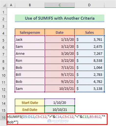
3. Using SUMIFS with Multiple Columns and Date Criteria
Let's say we have a table with the following columns: Date, Region, Product, Sales. We want to sum the sales for the North region and Product A in the month of January 2022.
| Date | Region | Product | Sales |
|---|---|---|---|
| 2022-01-01 | North | Product A | 100 |
| 2022-01-15 | North | Product B | 200 |
| 2022-02-01 | South | Product A | 300 |
| 2022-02-15 | South | Product B | 400 |
Using the SUMIFS function, we can achieve this as follows:
=SUMIFS(D:D, A:A, ">="&DATE(2022,1,1), A:A, "<="&DATE(2022,1,31), B:B, "North", C:C, "Product A")
This formula sums the values in column D (Sales) where the value in column A (Date) is between January 1, 2022, and January 31, 2022, the value in column B (Region) is North, and the value in column C (Product) is Product A.

4. Using SUMIFS with Multiple Columns and OR Criteria
Suppose we want to sum the sales for the North region and Product A or Product B. We can use the OR criteria by separating the criteria ranges and criteria with a comma.
=SUMIFS(C:C, A:A, "North", (B:B, "Product A"), (B:B, "Product B"))
However, the above formula will not work directly, as SUMIFS function does not directly support OR logic. Instead, we can use the SUMIFS function twice and add the results:
=SUMIFS(C:C, A:A, "North", B:B, "Product A") + SUMIFS(C:C, A:A, "North", B:B, "Product B")
This formula sums the values in column C (Sales) where the value in column A (Region) is North and the value in column B (Product) is either Product A or Product B.
5. Using SUMIFS with Multiple Columns and Dynamic Criteria
Let's say we have a table with the following columns: Region, Product, Sales, and we want to sum the sales for a specific region and product selected from a dropdown list.
| Region | Product | Sales |
|---|---|---|
| North | Product A | 100 |
| North | Product B | 200 |
| South | Product A | 300 |
| South | Product B | 400 |
We can use the SUMIFS function with dynamic criteria as follows:
=SUMIFS(C:C, A:A, A2, B:B, B2)
Assuming the dropdown list for the region is in cell A2 and the dropdown list for the product is in cell B2. This formula sums the values in column C (Sales) where the value in column A (Region) is equal to the selected value in cell A2 and the value in column B (Product) is equal to the selected value in cell B2.

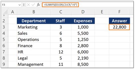
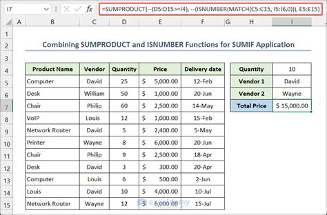
Gallery of SUMIFS Examples
SUMIFS Function Examples


In conclusion, using the SUMIFS function with multiple columns in Excel can significantly enhance your data analysis capabilities. By mastering the five ways to use SUMIFS with multiple columns, you can easily sum values based on multiple conditions applied to different columns. Remember to use the correct syntax, and don't hesitate to experiment with different criteria and ranges to achieve the desired results.
We hope this article has been informative and helpful in your Excel journey. If you have any questions or need further clarification, please don't hesitate to ask. Share your thoughts and experiences with the SUMIFS function in the comments section below.
