5 Ways To Master Excel Two Column Lookup

In the world of data analysis, Microsoft Excel is an indispensable tool for professionals and individuals alike. Among its numerous features, the two-column lookup is a crucial function that enables users to retrieve specific data from a table based on two criteria. However, mastering this skill can be challenging, especially for those new to Excel. In this article, we will explore five ways to master the two-column lookup in Excel, making it easier for you to work with complex data sets.

Understanding the Two-Column Lookup

Before diving into the methods, it's essential to understand the basics of the two-column lookup. This function involves searching for a value in two columns of a table and returning a corresponding value from another column. The two-column lookup is particularly useful when working with large datasets, where a single column lookup may not be sufficient.

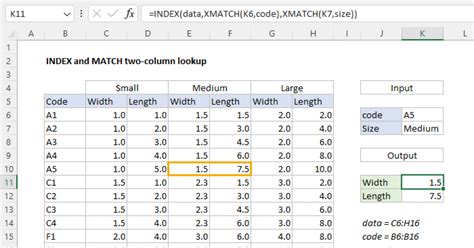
Method 1: Using the INDEX-MATCH Function

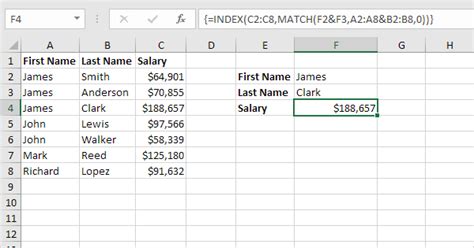
The INDEX-MATCH function is a powerful combination that can be used for two-column lookups. The INDEX function returns a value at a specific position in a range, while the MATCH function returns the position of a value in a range.

To use the INDEX-MATCH function for a two-column lookup:

• Select the cell where you want to display the result.
• Type =INDEX(range,MATCH(1,(range1=lookup_value1)*(range2=lookup_value2),0)), where range is the range of cells containing the values you want to return, range1 and range2 are the ranges of cells containing the lookup values, and lookup_value1 and lookup_value2 are the values you want to look up.
• Press Enter to get the result.

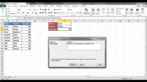
For example, if you have a table with names in column A, ages in column B, and cities in column C, and you want to find the city of a person with a specific name and age, you can use the following formula:

=INDEX(C:C,MATCH(1,(A:A="John")*(B:B=25),0))

Method 2: Using the VLOOKUP Function with Multiple Criteria

The VLOOKUP function is a popular choice for lookups in Excel, and it can be modified to work with multiple criteria. To use VLOOKUP for a two-column lookup:

• Select the cell where you want to display the result.
• Type =VLOOKUP(lookup_value1,range,2,FALSE)*VLOOKUP(lookup_value2,range,2,FALSE), where lookup_value1 and lookup_value2 are the values you want to look up, and range is the range of cells containing the values you want to return.
• Press Enter to get the result.

However, this method has limitations, as it can only return values from the second column of the range.

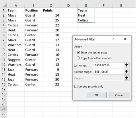
Method 3: Using the FILTER Function

The FILTER function is a relatively new addition to Excel, introduced in Excel 2019. It allows you to filter a range of cells based on multiple criteria.

To use the FILTER function for a two-column lookup:

• Select the cell where you want to display the result.
• Type =FILTER(range,(range1=lookup_value1)*(range2=lookup_value2)), where range is the range of cells containing the values you want to return, range1 and range2 are the ranges of cells containing the lookup values, and lookup_value1 and lookup_value2 are the values you want to look up.
• Press Enter to get the result.

For example, if you have a table with names in column A, ages in column B, and cities in column C, and you want to find the city of a person with a specific name and age, you can use the following formula:

=FILTER(C:C,(A:A="John")*(B:B=25))

Method 4: Using Power Query

Power Query is a powerful tool in Excel that allows you to manipulate and analyze data. You can use Power Query to perform a two-column lookup by creating a custom function.

To use Power Query for a two-column lookup:

• Go to the "Data" tab in the ribbon.
• Click on "New Query" and then "From Other Sources" and select "Blank Query".
• In the Query Editor, click on "Add Column" and then "Custom Column".
• Type =Table.Filter(range,each [Column1]=lookup_value1 and [Column2]=lookup_value2) and click "OK", where range is the range of cells containing the values you want to return, Column1 and Column2 are the column names containing the lookup values, and lookup_value1 and lookup_value2 are the values you want to look up.
• Click on "Load" to load the result into a new table.

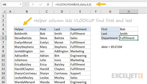
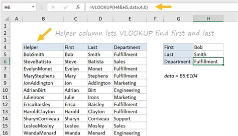
Method 5: Using a Helper Column

A helper column is a temporary column that you can use to perform a two-column lookup. You can create a helper column by concatenating the two lookup columns and then using the VLOOKUP function to return the result.

To use a helper column for a two-column lookup:

• Create a new column next to the range of cells containing the values you want to return.
• Type =A2&B2 in the first cell of the helper column, where A2 and B2 are the cells containing the lookup values.
• Copy the formula down to the rest of the cells in the helper column.
• Use the VLOOKUP function to return the result, using the helper column as the lookup range.

For example, if you have a table with names in column A, ages in column B, and cities in column C, and you want to find the city of a person with a specific name and age, you can use the following formula:

=VLOOKUP("John25",E:E,2,FALSE)

Gallery of Excel Two Column Lookup Examples

Excel Two Column Lookup Examples

Conclusion

Mastering the two-column lookup in Excel can be a game-changer for data analysis and manipulation. By using one of the five methods outlined in this article, you can efficiently retrieve data from a table based on two criteria. Whether you're a beginner or an advanced user, practicing these methods will help you become more proficient in using Excel for data analysis.