3 Ways To Unhide Top Rows In Excel

Have you ever worked on an Excel spreadsheet only to find that the top rows have disappeared from view? This can be frustrating, especially if you're trying to reference important data or headers. Fortunately, there are a few ways to unhide top rows in Excel. In this article, we'll explore three methods to help you regain visibility of your hidden rows.

Method 1: Unhide Rows using the Row Header

The first method is to use the row header to unhide the top rows. To do this:

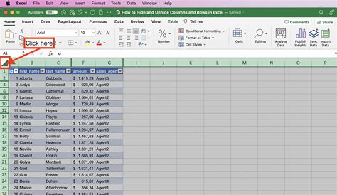
Select the row below the hidden rows by clicking on the row number in the row header.
Go to the "Home" tab in the Excel ribbon.
Click on the "Format" button in the "Cells" group.
Select "Row" from the drop-down menu.
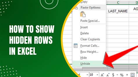
Click on "Unhide" from the sub-menu.

This method will unhide all rows above the selected row. If you want to unhide a specific range of rows, you can select the range by clicking and dragging on the row numbers in the row header, and then follow the same steps.

Method 2: Use the Excel Formula Bar

Another way to unhide top rows in Excel is to use the formula bar. To do this:

Select the cell in the top row that you want to unhide.
Go to the formula bar and type =ROW(A1) (assuming the top row is row 1).
Press Enter to apply the formula.
The formula will return the row number, which will automatically unhide the row.

This method is useful if you know the exact row number that you want to unhide. You can also use this method to unhide multiple rows by selecting a range of cells and applying the formula.

Method 3: Use Excel Shortcuts

The final method is to use Excel shortcuts to unhide top rows. To do this:

Press Ctrl + 9 to hide the selected rows.
Press Ctrl + Shift + 9 to unhide the selected rows.

If you want to unhide all rows in the worksheet, you can press Ctrl + A to select all cells, and then press Ctrl + Shift + 9 to unhide all rows.

Common Reasons for Hidden Top Rows in Excel

Before we dive deeper into the solutions, let's explore some common reasons why top rows might be hidden in Excel:

Accidental hiding: It's easy to accidentally hide rows in Excel, especially if you're working with a large dataset. If you select a range of cells and press Ctrl + 9, the rows will be hidden.
Conditional formatting: If you've applied conditional formatting to a range of cells, it's possible that the formatting has hidden the top rows.
VBA macros: If you've created a VBA macro to automate tasks in Excel, it's possible that the macro has hidden the top rows.

Troubleshooting Hidden Top Rows in Excel

If you're having trouble unhiding top rows in Excel, here are some troubleshooting steps to try:

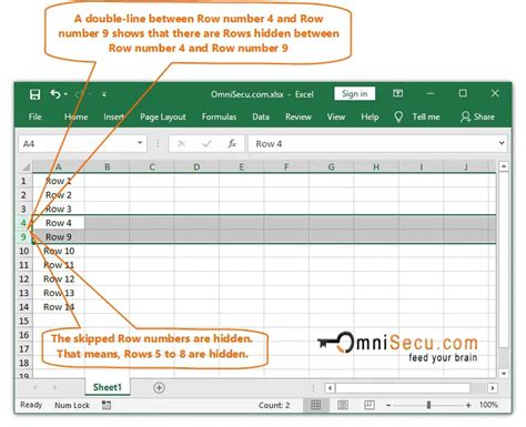
Check the row header: Make sure that the row header is visible and not frozen. If the row header is frozen, you won't be able to unhide the top rows.
Check for conditional formatting: If you've applied conditional formatting to a range of cells, check the formatting rules to see if they're hiding the top rows.
Check for VBA macros: If you've created a VBA macro, check the code to see if it's hiding the top rows.

Best Practices for Working with Hidden Rows in Excel

Here are some best practices for working with hidden rows in Excel:

Use clear headings: Use clear and descriptive headings to identify the data in your spreadsheet.
Use formatting: Use formatting to make your data stand out, but avoid using formatting to hide rows.
Use VBA macros carefully: If you're using VBA macros to automate tasks in Excel, make sure to test them carefully to avoid hiding rows unintentionally.

Conclusion

Hidden top rows in Excel can be frustrating, but there are several ways to unhide them. By using the row header, Excel formula bar, or Excel shortcuts, you can regain visibility of your hidden rows. Remember to troubleshoot common issues and follow best practices for working with hidden rows in Excel.