Finding a specific value within a range of numbers in Excel can be a common task, especially when working with large datasets. Whether you're looking for a value that falls between two specific numbers or trying to identify values that meet certain criteria, Excel provides various functions and techniques to help you achieve this goal. In this article, we'll explore five methods to find an Excel value between two numbers, highlighting their uses, benefits, and how to apply them in different scenarios.
Method 1: Using the IF Function
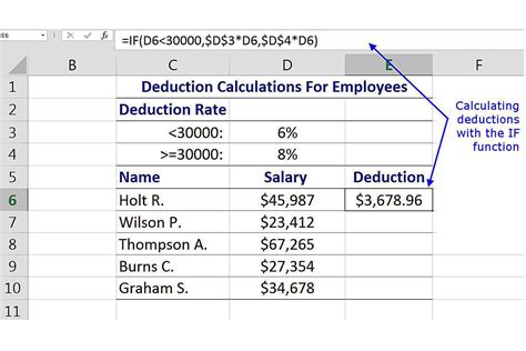
The IF function is one of the most commonly used functions in Excel for conditional statements. It can be utilized to check if a value falls within a specified range. The syntax of the IF function is:
IF(logical_test, [value_if_true], [value_if_false])
To find a value between two numbers, you would use the formula:
=IF(AND(A1>=lower_limit, A1<=upper_limit), "Within Range", "Outside Range")
In this formula, A1 is the cell containing the value to check, lower_limit and upper_limit are the minimum and maximum values of the range, respectively.
Example Use Case:
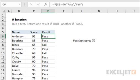
Suppose you have a list of exam scores in column A and you want to check if a score is between 70 and 90. You can use the IF function to return "Pass" if the score is within this range and "Fail" otherwise.
| Score |
|---|
| 85 |
| 67 |
| 92 |
| 78 |
Using the formula =IF(AND(A2>=70, A2<=90), "Pass", "Fail") in column B, you'll get the following results:
| Score | Result |
|---|---|
| 85 | Pass |
| 67 | Fail |
| 92 | Fail |
| 78 | Pass |
Method 2: Using the FILTER Function (Excel 365 and Later)

The FILTER function, introduced in Excel 365, allows you to filter a range of data based on a specified condition. The syntax is:
FILTER(range, include, [if_empty])
To find values between two numbers, you can use the formula:
=FILTER(A:A, (A:A>=lower_limit) * (A:A<=upper_limit))
This formula filters the values in column A to include only those that are greater than or equal to lower_limit and less than or equal to upper_limit.
Example Use Case:
Using the same example as above, if you want to filter the scores to show only those between 70 and 90, you can use the FILTER function in a new column:
| Score |
|---|
| 85 |
| 67 |
| 92 |
| 78 |
Using the formula =FILTER(A:A, (A:A>=70) * (A:A<=90)) in column C, you'll get the following filtered results:
| Score |
|---|
| 85 |
| 78 |
Method 3: Using Conditional Formatting

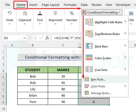
Conditional formatting allows you to highlight cells that meet specific conditions. To find values between two numbers, you can set up a rule to format cells based on a formula.
- Select the range of cells you want to format.
- Go to the Home tab > Conditional Formatting > New Rule.
- Choose "Use a formula to determine which cells to format."
- Enter the formula:
=AND(A1>=lower_limit, A1<=upper_limit) - Click Format to select the desired formatting.
- Click OK.
Example Use Case:
To highlight scores between 70 and 90, you can apply conditional formatting to the range A1:A10:
| Score |
|---|
| 85 |
| 67 |
| 92 |
| 78 |
After applying the rule, cells with scores between 70 and 90 will be highlighted.
Method 4: Using VLOOKUP
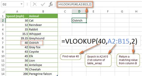
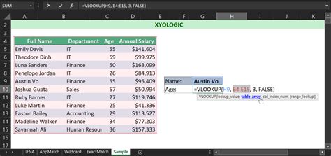
VLOOKUP is a powerful function that allows you to search for a value in a table and return a corresponding value from another column. While not directly designed to find values between two numbers, you can use VLOOKUP with some creativity.
- Create a table with the lower and upper limits in one column and the corresponding values in another column.
- Use the VLOOKUP function to search for the value in the first column and return the corresponding value in the second column.
Example Use Case:
Suppose you have a table with score ranges and corresponding grades:
| Score Range | Grade |
|---|---|
| 70-80 | C |
| 81-90 | B |
| 91-100 | A |
To find the grade for a score of 85, you can use the VLOOKUP function:
=VLOOKUP(A2, score_range_table, 2, FALSE)
This formula searches for the score in the first column of the table and returns the corresponding grade in the second column.
Method 5: Using INDEX-MATCH
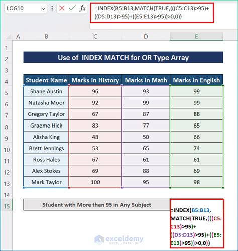
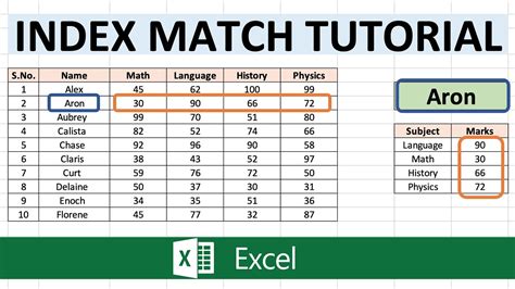
The INDEX-MATCH function combination is a more flexible and powerful alternative to VLOOKUP. It allows you to search for a value in a range and return a corresponding value from another range.
- Use the MATCH function to find the relative position of the value in the range.
- Use the INDEX function to return the corresponding value from another range.
Example Use Case:
Using the same example as above, you can use the INDEX-MATCH function to find the grade for a score of 85:
=INDEX(grade_range, MATCH(A2, score_range, 0))
This formula searches for the score in the first range and returns the corresponding grade from the second range.
Excel Value Between Two Numbers Image Gallery



We hope this comprehensive guide has helped you learn how to find Excel values between two numbers using various methods. Whether you're a beginner or an advanced user, mastering these techniques will improve your productivity and data analysis skills. Remember to practice and experiment with different functions and formulas to become proficient in using Excel to its full potential.
What's your favorite method for finding values between two numbers in Excel? Share your thoughts and experiences in the comments section below. Don't forget to share this article with your colleagues and friends who might benefit from learning these techniques.
