5 Ways To Format Negative Numbers In Excel

Formatting negative numbers in Excel is a common task that can enhance the readability and professionalism of your spreadsheets. Proper formatting helps to differentiate negative numbers from positive ones, making it easier to analyze and understand your data. In this article, we will explore five different ways to format negative numbers in Excel, along with practical examples and explanations.

Understanding Default Negative Number Formatting

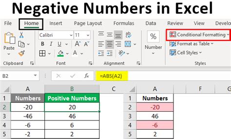
Before we dive into custom formatting options, let's take a look at how Excel handles negative numbers by default. When you enter a negative number in a cell, Excel will display it with a minus sign (-) preceding the number. This is the most straightforward way to indicate a negative value. However, you may want to change the formatting to better suit your needs.

Method 1: Using the Accounting Format

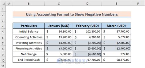
The Accounting format is a popular choice for formatting negative numbers in Excel. This format encloses negative numbers in parentheses, making them stand out from positive numbers. To apply the Accounting format:

1. Select the cells containing the negative numbers you want to format.
2. Go to the Home tab in the Excel ribbon.
3. Click on the Number group and select the Accounting button.
4. Choose the desired currency symbol and decimal places.

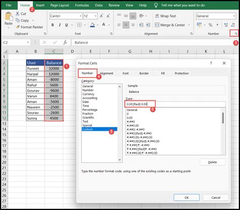
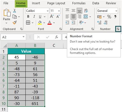
Method 2: Using Custom Number Formatting

If you want more control over the formatting of negative numbers, you can use Custom Number Formatting. This method allows you to create a custom format that suits your specific needs. To apply a custom format:

1. Select the cells containing the negative numbers you want to format.
2. Go to the Home tab in the Excel ribbon.
3. Click on the Number group and select the Custom button.
4. In the Format Cells dialog box, enter a custom format code in the Type field. For example, to display negative numbers in red, you can use the following code: #,##0.00;[Red]#,##0.00

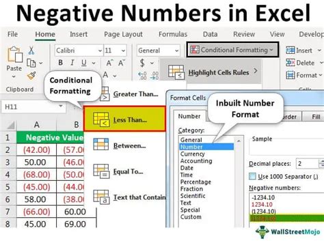
Method 3: Using Conditional Formatting

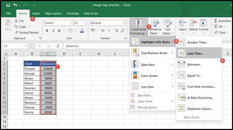
Conditional Formatting is a powerful tool in Excel that allows you to format cells based on specific conditions. You can use this feature to highlight negative numbers in a different color or format. To apply Conditional Formatting:

1. Select the cells containing the negative numbers you want to format.
2. Go to the Home tab in the Excel ribbon.
3. Click on the Conditional Formatting button in the Styles group.
4. Select the "Highlight Cells Rules" option and choose "Less Than".
5. Set the value to 0 and choose a format from the drop-down menu.

Method 4: Using Number Formatting Codes

Number Formatting Codes are a series of codes that you can use to create custom number formats in Excel. These codes can be used to format negative numbers in a specific way. To apply a Number Formatting Code:

1. Select the cells containing the negative numbers you want to format.
2. Go to the Home tab in the Excel ribbon.
3. Click on the Number group and select the Custom button.
4. In the Format Cells dialog box, enter a Number Formatting Code in the Type field. For example, to display negative numbers with a minus sign and parentheses, you can use the following code: #,##0.00;(#,##0.00)

Method 5: Using VBA Macros

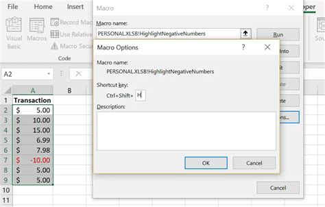
If you want to automate the formatting of negative numbers in Excel, you can use VBA Macros. VBA Macros are small programs that can be written to perform specific tasks in Excel. To create a VBA Macro for formatting negative numbers:

1. Open the Visual Basic Editor by pressing Alt + F11 or by navigating to Developer > Visual Basic.
2. Create a new module by clicking Insert > Module.
3. Write a VBA Macro code to format negative numbers. For example: Sub FormatNegativeNumbers() Range("A1:A10").Select Selection.NumberFormat = "#,##0.00;(#,##0.00)" End Sub

Gallery of Negative Number Formatting Examples

Negative Number Formatting Examples

Conclusion

Formatting negative numbers in Excel is an essential task that can improve the readability and professionalism of your spreadsheets. By using one of the five methods outlined in this article, you can create custom formats that suit your specific needs. Whether you prefer the Accounting format, Custom Number Formatting, Conditional Formatting, Number Formatting Codes, or VBA Macros, there is a method that can help you format negative numbers effectively.