
Are you tired of manually creating quadrant graphs in Excel? Do you struggle to effectively visualize and analyze your data? Look no further! In this article, we will guide you through the process of creating a 4-quadrant graph in Excel in just 5 easy steps.
Understanding the Importance of Quadrant Graphs
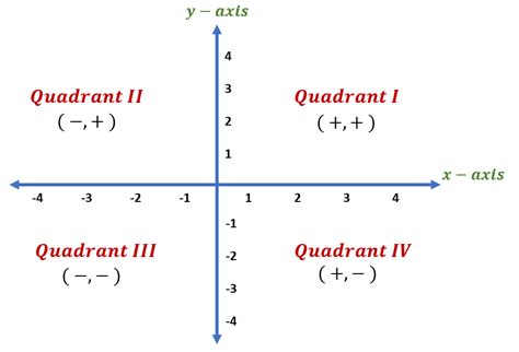
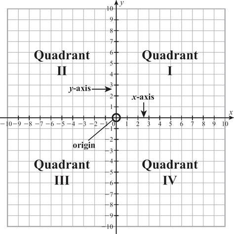
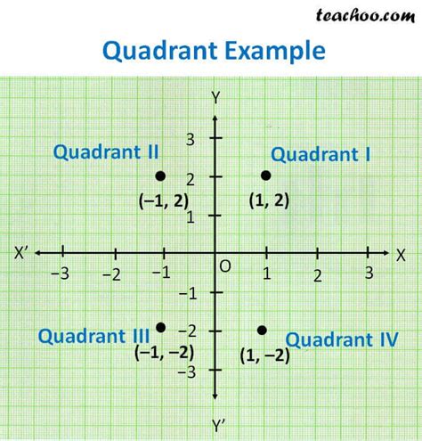
Before we dive into the steps, let's quickly discuss the importance of quadrant graphs. Quadrant graphs, also known as scatter plots or 2x2 matrices, are a powerful visualization tool used to analyze and compare data points across two variables. They help identify patterns, trends, and correlations between variables, making it easier to make informed decisions.
Step 1: Prepare Your Data
To create a 4-quadrant graph, you'll need to prepare your data. This involves setting up two columns of data in your Excel spreadsheet. The first column should represent the x-axis variable, while the second column represents the y-axis variable. Ensure that your data is organized in a table format, with headers in the first row and data points in the subsequent rows.
Step 2: Create a Scatter Plot
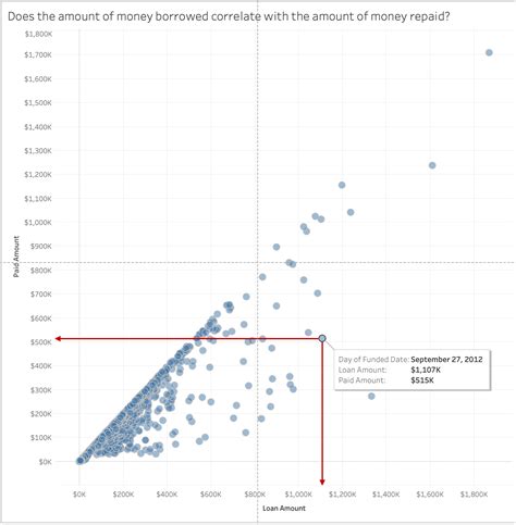
To create a scatter plot, select your data range, including headers. Go to the "Insert" tab in the Excel ribbon and click on "Scatter" in the "Charts" group. Choose the "Scatter with only markers" option. This will create a basic scatter plot with your data points.
Step 3: Add Axis Labels and Titles
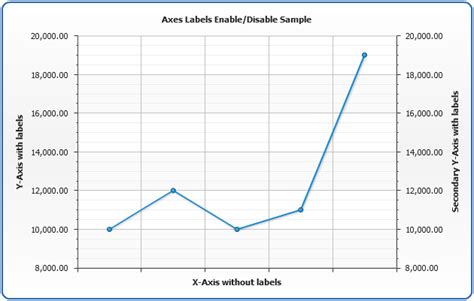
To make your graph more readable, add axis labels and titles. Right-click on the x-axis and select "Format Axis." In the "Format Axis" pane, enter a title for the x-axis. Repeat this process for the y-axis. You can also add a chart title by clicking on the "Chart Title" button in the "Chart Tools" tab.
Step 4: Create Quadrant Lines
To divide your graph into four quadrants, you'll need to create two lines: a vertical line for the x-axis and a horizontal line for the y-axis. To create a vertical line, go to the "Insert" tab and click on "Shapes." Select the "Line" option and draw a vertical line at the desired x-axis value. Repeat this process for the horizontal line, drawing it at the desired y-axis value.
Step 5: Format and Customize
The final step is to format and customize your graph. You can adjust the line colors, styles, and widths to make your graph more visually appealing. You can also add data labels, adjust the scale, and change the background color to enhance the overall appearance of your graph.
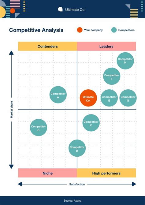
Gallery of Quadrant Graph Examples
Quadrant Graph Examples


Conclusion
Creating a 4-quadrant graph in Excel is a simple and effective way to visualize and analyze your data. By following these 5 easy steps, you can create a quadrant graph that helps you identify patterns, trends, and correlations between variables. Don't forget to format and customize your graph to make it more visually appealing and effective in communicating your findings.
Take Action!
Try creating a 4-quadrant graph in Excel today and see how it can help you gain insights into your data. Share your experiences and tips in the comments below. If you have any questions or need further assistance, feel free to ask!