5 Ways To Lookup Multiple Criteria In Google Sheets

Managing and analyzing data in Google Sheets can be a daunting task, especially when dealing with large datasets. One of the most common challenges users face is looking up values based on multiple criteria. Fortunately, Google Sheets provides several functions and techniques to help you achieve this. In this article, we will explore five ways to lookup multiple criteria in Google Sheets.

Understanding the Importance of Lookup Functions

Lookup functions are essential in Google Sheets, as they enable you to search for specific values within a dataset. These functions are particularly useful when working with large datasets, where manual searches can be time-consuming and prone to errors. By using lookup functions, you can quickly and accurately retrieve data based on one or more criteria.

Method 1: Using the FILTER Function

The FILTER function is one of the most versatile and powerful lookup functions in Google Sheets. It allows you to filter a dataset based on multiple criteria, making it an ideal choice for complex lookup tasks. The syntax for the FILTER function is:

FILTER(range, condition1, [condition2], …)

Where:

• range is the range of cells you want to filter.
• condition1, condition2, etc. are the conditions you want to apply to the filter.

For example, suppose you have a dataset with the following columns: Name, Age, Country. You can use the FILTER function to retrieve all rows where the Age is greater than 25 and the Country is "USA":

=FILTER(A2:C10, B2:B10 > 25, C2:C10 = "USA")

This formula will return all rows where the Age is greater than 25 and the Country is "USA".

Method 2: Using the INDEX and MATCH Functions

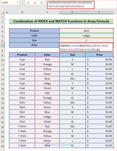
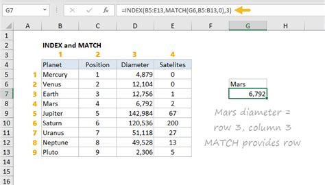
The INDEX and MATCH functions are two of the most popular lookup functions in Google Sheets. While they can be used separately, combining them provides a powerful way to lookup multiple criteria. The syntax for the INDEX and MATCH functions is:

INDEX(range, MATCH(lookup_value, range, [match_type])

Where:

• range is the range of cells you want to search.
• lookup_value is the value you want to search for.
• match_type is the type of match you want to perform (e.g., exact match, approximate match).

For example, suppose you have a dataset with the following columns: Name, Age, Country. You can use the INDEX and MATCH functions to retrieve the Age of a person with a specific Name and Country:

=INDEX(B2:B10, MATCH(1, (A2:A10 = "John") * (C2:C10 = "USA"), 0))

This formula will return the Age of the person named "John" from the "USA".

Method 3: Using the VLOOKUP Function with Multiple Criteria

The VLOOKUP function is a popular lookup function in Google Sheets. While it is typically used to search for a single value, you can also use it to search for multiple criteria by combining it with other functions, such as the & operator. The syntax for the VLOOKUP function is:

VLOOKUP(lookup_value, range, col_index, [range_lookup])

Where:

• lookup_value is the value you want to search for.
• range is the range of cells you want to search.
• col_index is the column index of the value you want to retrieve.
• range_lookup is the type of match you want to perform (e.g., exact match, approximate match).

For example, suppose you have a dataset with the following columns: Name, Age, Country. You can use the VLOOKUP function with multiple criteria to retrieve the Age of a person with a specific Name and Country:

=VLOOKUP(A2 & "*" & C2, A2:C10, 2, FALSE)

This formula will return the Age of the person with the Name in cell A2 and the Country in cell C2.

Method 4: Using the Query Function

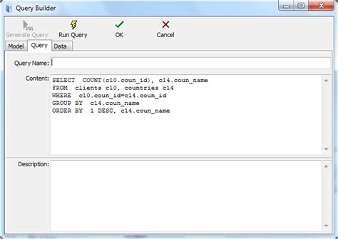
The Query function is a powerful function in Google Sheets that allows you to perform complex queries on your data. It uses a SQL-like syntax to define the query, making it easy to filter and retrieve data based on multiple criteria. The syntax for the Query function is:

QUERY(range, query, [headers])

Where:

• range is the range of cells you want to query.
• query is the SQL-like query you want to perform.
• headers is the number of header rows in the range.

For example, suppose you have a dataset with the following columns: Name, Age, Country. You can use the Query function to retrieve all rows where the Age is greater than 25 and the Country is "USA":

=QUERY(A2:C10, "SELECT * WHERE B > 25 AND C = 'USA'")

This formula will return all rows where the Age is greater than 25 and the Country is "USA".

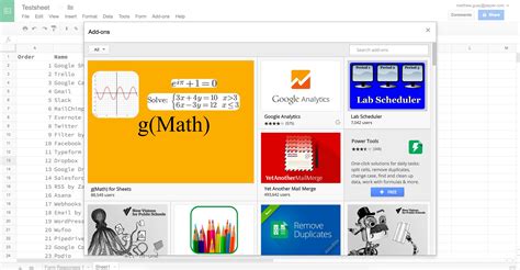
Method 5: Using the Google Sheets Add-on

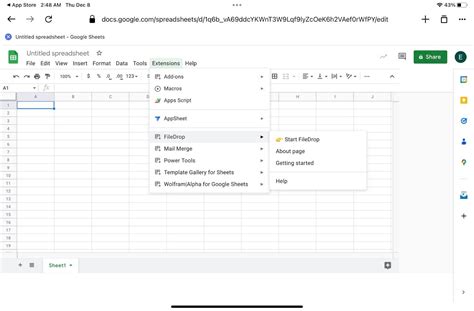
If you're not comfortable using formulas or want a more user-friendly solution, you can use the Google Sheets add-on. The add-on provides a simple and intuitive interface to lookup multiple criteria. To use the add-on, follow these steps:

1. Open your Google Sheet.
2. Click on the "Add-ons" menu.
3. Search for "Lookup" and click on the result.
4. Click on the "Install" button.
5. Follow the prompts to authorize the add-on.

Once installed, you can use the add-on to lookup multiple criteria by following these steps:

1. Select the range of cells you want to search.
2. Click on the "Lookup" button in the add-on menu.
3. Enter the criteria you want to search for.
4. Click on the "Search" button.

The add-on will return the results based on the criteria you specified.

Gallery of Lookup Functions in Google Sheets

Lookup Functions in Google Sheets

In conclusion, looking up multiple criteria in Google Sheets can be a challenging task, but with the right functions and techniques, you can achieve accurate and efficient results. By using the FILTER, INDEX and MATCH, VLOOKUP, Query, and Google Sheets add-on methods, you can simplify your lookup tasks and focus on analyzing and interpreting your data.