Google Sheets Vlookup From Another Tab Made Easy

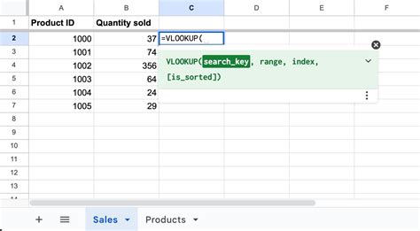
If you're a frequent user of Google Sheets, you know how powerful and versatile it can be for managing and analyzing data. One of the most useful functions in Google Sheets is VLOOKUP, which allows you to search for a value in a table and return a corresponding value from another column. However, using VLOOKUP to retrieve data from another tab can be a bit tricky. In this article, we'll show you how to use VLOOKUP to pull data from another tab in Google Sheets.

Why Use VLOOKUP from Another Tab?

Before we dive into the details, let's talk about why you might want to use VLOOKUP to retrieve data from another tab. Suppose you have a Google Sheet with multiple tabs, each containing different sets of data. You might have a tab for customer information, a tab for order history, and a tab for product details. Using VLOOKUP, you can easily retrieve data from one tab and display it in another tab, making it easier to analyze and report on your data.

The Basics of VLOOKUP

Before we explore how to use VLOOKUP to retrieve data from another tab, let's review the basics of the function. VLOOKUP is a function that searches for a value in a table and returns a corresponding value from another column. The syntax for VLOOKUP is as follows:

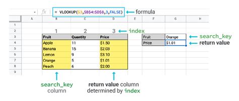
VLOOKUP(search_key, range, index, [is_exact_match])

• search_key is the value you want to search for
• range is the range of cells that contains the data you want to search
• index is the column number that contains the value you want to return
• [is_exact_match] is an optional argument that specifies whether you want an exact match or not

Using VLOOKUP to Retrieve Data from Another Tab

Now that we've reviewed the basics of VLOOKUP, let's talk about how to use it to retrieve data from another tab. The process is similar to using VLOOKUP within the same tab, but you need to specify the tab name and range of cells that contains the data you want to search.

Here's an example:

Suppose you have a Google Sheet with two tabs: "Customers" and "Orders". The "Customers" tab contains a list of customer names and IDs, while the "Orders" tab contains a list of orders with corresponding customer IDs. You want to use VLOOKUP to retrieve the customer name from the "Customers" tab and display it in the "Orders" tab.

Here's the formula you would use:

=VLOOKUP(A2, Customers!A:B, 2, FALSE)

• A2 is the cell that contains the customer ID you want to search for
• Customers!A:B is the range of cells that contains the customer data, including the customer IDs and names
• 2 is the column number that contains the customer name
• FALSE specifies that you want an exact match

How to Specify the Tab Name and Range

When using VLOOKUP to retrieve data from another tab, you need to specify the tab name and range of cells that contains the data you want to search. To do this, you can use the following syntax:

TabName!Range

• TabName is the name of the tab that contains the data you want to search
• Range is the range of cells that contains the data you want to search

For example, if you want to search for data in a tab named "Customers", you would use the following syntax:

Customers!A:B

This specifies that you want to search for data in columns A and B of the "Customers" tab.

Tips and Tricks

Here are a few tips and tricks to keep in mind when using VLOOKUP to retrieve data from another tab:

• Make sure to specify the correct tab name and range of cells that contains the data you want to search.
• Use the ! symbol to separate the tab name from the range of cells.
• Use the $ symbol to lock the tab name and range of cells, so that they don't change when you copy the formula to other cells.
• Use the FALSE argument to specify that you want an exact match.

Common Errors

Here are a few common errors to watch out for when using VLOOKUP to retrieve data from another tab:

• Forgetting to specify the tab name and range of cells that contains the data you want to search.
• Using the wrong syntax to specify the tab name and range of cells.
• Forgetting to use the ! symbol to separate the tab name from the range of cells.
• Forgetting to use the FALSE argument to specify that you want an exact match.

Gallery of Google Sheets Vlookup Examples

Google Sheets Vlookup Examples

Frequently Asked Questions

Here are a few frequently asked questions about using VLOOKUP to retrieve data from another tab:

Q: What is the syntax for using VLOOKUP to retrieve data from another tab? A: The syntax is =VLOOKUP(search_key, TabName!Range, index, [is_exact_match]).

Q: How do I specify the tab name and range of cells that contains the data I want to search? A: You can use the syntax TabName!Range, where TabName is the name of the tab and Range is the range of cells that contains the data you want to search.

Q: What is the ! symbol used for in the VLOOKUP formula? A: The ! symbol is used to separate the tab name from the range of cells.

Q: How do I use the FALSE argument in the VLOOKUP formula? A: You can use the FALSE argument to specify that you want an exact match.

We hope this article has helped you learn how to use VLOOKUP to retrieve data from another tab in Google Sheets. With this powerful function, you can easily analyze and report on your data, even if it's spread across multiple tabs.