
In Google Sheets, the VLOOKUP function is a powerful tool for searching and retrieving data from a table. However, the traditional VLOOKUP function has its limitations, particularly when it comes to looking up multiple values. Fortunately, there are several workarounds and alternatives that allow you to VLOOKUP multiple values in Google Sheets. In this article, we'll explore five methods to achieve this, along with practical examples and step-by-step instructions.
Understanding the Traditional VLOOKUP Function
Before diving into the methods for VLOOKUPing multiple values, let's quickly review the traditional VLOOKUP function syntax:
VLOOKUP(search_key, range, index, [is_exact_match])
search_key: the value you want to search forrange: the range of cells that contains the dataindex: the column number that contains the value you want to return[is_exact_match]: an optional parameter that specifies whether you want an exact match (TRUE) or an approximate match (FALSE)
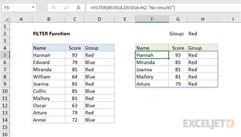
Method 1: Using the FILTER Function
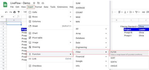
One of the most straightforward ways to VLOOKUP multiple values is by using the FILTER function. The FILTER function allows you to filter a range of cells based on a condition, which can include multiple values.
Example:
Suppose you have a table with employee data, and you want to retrieve the names of employees who work in either the Sales or Marketing department.
| Employee ID | Name | Department |
|---|---|---|
| 101 | John Smith | Sales |
| 102 | Jane Doe | Marketing |
| 103 | Bob Johnson | Sales |
| 104 | Alice Brown | Marketing |
You can use the following formula:
=FILTER(A:B, (C:C = "Sales") + (C:C = "Marketing"))
This formula will return the names of employees who work in either the Sales or Marketing department.
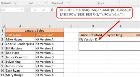
Method 2: Using the INDEX and MATCH Functions
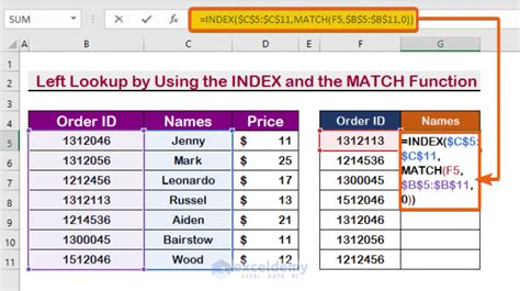
Another approach is to use the INDEX and MATCH functions in combination. The INDEX function returns a value at a specified position, while the MATCH function returns the relative position of a value within a range.
Example:
Suppose you have a table with student data, and you want to retrieve the grades of students who scored either 90 or 95 on a test.
| Student ID | Name | Grade |
|---|---|---|
| 201 | Emily Chen | 90 |
| 202 | David Lee | 95 |
| 203 | Sophia Patel | 80 |
| 204 | Michael Kim | 90 |
You can use the following formula:
=INDEX(C:C, MATCH(1, (B:B = 90) + (B:B = 95), 0))
This formula will return the grades of students who scored either 90 or 95.
Method 3: Using the Query Function
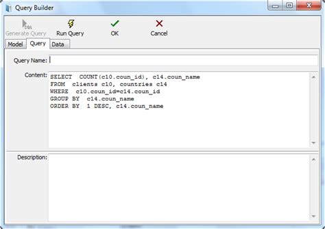
The Query function is a powerful tool for querying and manipulating data in Google Sheets. You can use it to VLOOKUP multiple values by specifying a query that filters the data based on multiple conditions.
Example:
Suppose you have a table with product data, and you want to retrieve the prices of products that belong to either the Electronics or Fashion category.
| Product ID | Name | Category | Price |
|---|---|---|---|
| 301 | iPhone | Electronics | 999 |
| 302 | Samsung TV | Electronics | 1299 |
| 303 | Levi's Jeans | Fashion | 79 |
| 304 | Nike Shoes | Fashion | 129 |
You can use the following formula:
=QUERY(A:D, "SELECT D WHERE C = 'Electronics' OR C = 'Fashion'")
This formula will return the prices of products that belong to either the Electronics or Fashion category.
Method 4: Using the Array Formula
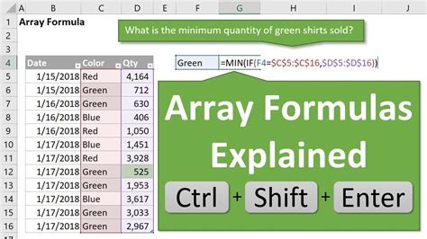
Array formulas are a powerful feature in Google Sheets that allows you to perform calculations on arrays of data. You can use an array formula to VLOOKUP multiple values by creating an array of search keys and then using the VLOOKUP function to retrieve the corresponding values.
Example:
Suppose you have a table with customer data, and you want to retrieve the addresses of customers who live in either New York or California.
| Customer ID | Name | Address |
|---|---|---|
| 401 | John Smith | 123 Main St, New York |
| 402 | Jane Doe | 456 Elm St, California |
| 403 | Bob Johnson | 789 Oak St, New York |
| 404 | Alice Brown | 321 Pine St, California |
You can use the following formula:
=ArrayFormula(VLOOKUP({"New York", "California"}, A:C, 2, FALSE))
This formula will return the addresses of customers who live in either New York or California.
Method 5: Using the XLOOKUP Function (Beta)
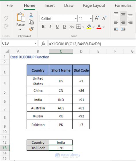
The XLOOKUP function is a new function in Google Sheets that allows you to search for a value in a range and return a corresponding value from another range. While it's still in beta, it's a promising alternative to the traditional VLOOKUP function.
Example:
Suppose you have a table with employee data, and you want to retrieve the department names of employees who work in either the Sales or Marketing department.
| Employee ID | Name | Department |
|---|---|---|
| 101 | John Smith | Sales |
| 102 | Jane Doe | Marketing |
| 103 | Bob Johnson | Sales |
| 104 | Alice Brown | Marketing |
You can use the following formula:
=XLOOKUP({"Sales", "Marketing"}, A:C, 2, FALSE)
This formula will return the department names of employees who work in either the Sales or Marketing department.
Gallery of VLOOKUP Multiple Values in Google Sheets
VLOOKUP Multiple Values in Google Sheets Image Gallery


In conclusion, VLOOKUPing multiple values in Google Sheets can be achieved through various methods, each with its own strengths and limitations. By understanding the different approaches and choosing the most suitable one for your specific needs, you can efficiently retrieve data and make informed decisions. We hope this article has been informative and helpful in your Google Sheets journey. If you have any questions or comments, please feel free to share them below!