Google Spreadsheet Conditional Formatting: Row Based On Cell

Google Spreadsheet Conditional Formatting is a powerful tool that allows you to highlight cells based on specific conditions, making it easier to analyze and understand your data. One of the most useful features of conditional formatting is the ability to apply formatting to an entire row based on the value of a single cell. In this article, we will explore how to use Google Spreadsheet Conditional Formatting to format a row based on a cell value.

Why Use Conditional Formatting?

Conditional formatting is a great way to visualize your data and make it more readable. By applying different formats to cells based on specific conditions, you can quickly identify trends, patterns, and outliers in your data. This can be especially useful when working with large datasets, where it can be difficult to identify important information at a glance.

How to Apply Conditional Formatting to a Row

To apply conditional formatting to a row based on a cell value, follow these steps:

1. Select the range of cells that you want to format. This can be a single row or multiple rows.
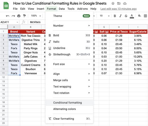
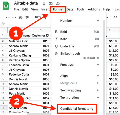
2. Go to the "Format" tab in the top menu.
3. Select "Conditional formatting" from the drop-down menu.
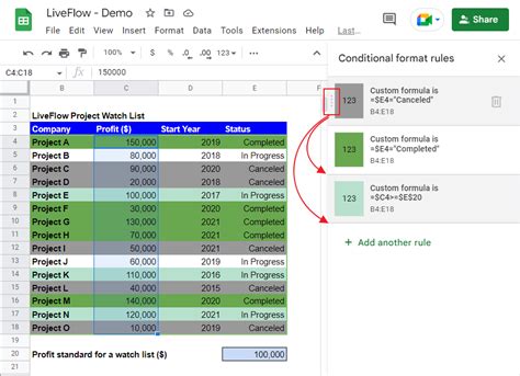
4. In the conditional formatting panel, select "Custom formula is" from the format cells if drop-down menu.
5. Enter the formula that you want to use to determine the formatting. For example, if you want to format a row based on the value in cell A1, you would enter the formula =A1>10.
6. Select the format that you want to apply to the row. You can choose from a variety of formats, including background color, font color, and borders.
7. Click "Done" to apply the formatting.

Using Relative References

When using conditional formatting to format a row based on a cell value, it's often necessary to use relative references. A relative reference is a reference to a cell that is relative to the current cell. For example, if you want to format a row based on the value in cell A1, you would use the relative reference A1 instead of the absolute reference $A$1.

Using Multiple Conditions

You can also use multiple conditions to format a row based on multiple cell values. To do this, follow these steps:

1. Select the range of cells that you want to format.
2. Go to the "Format" tab in the top menu.
3. Select "Conditional formatting" from the drop-down menu.
4. In the conditional formatting panel, select "Custom formula is" from the format cells if drop-down menu.
5. Enter the formula that you want to use to determine the formatting. For example, if you want to format a row based on the values in cells A1 and B1, you would enter the formula =AND(A1>10, B1<5).
6. Select the format that you want to apply to the row.
7. Click "Done" to apply the formatting.

Common Use Cases

There are many common use cases for conditional formatting in Google Spreadsheets. Here are a few examples:

• Highlighting important data: Use conditional formatting to highlight cells that contain important data, such as dates or deadlines.
• Identifying trends: Use conditional formatting to identify trends in your data, such as increases or decreases in sales or website traffic.
• Creating dashboards: Use conditional formatting to create dashboards that display key metrics and KPIs.

Tips and Tricks

Here are a few tips and tricks for using conditional formatting in Google Spreadsheets:

• Use named ranges: Use named ranges to make your formulas more readable and easier to maintain.
• Use relative references: Use relative references to make your formulas more flexible and easier to apply to multiple rows.
• Test your formulas: Test your formulas carefully to ensure that they are working as expected.

Google Spreadsheet Conditional Formatting Gallery

Conclusion

Google Spreadsheet Conditional Formatting is a powerful tool that allows you to highlight cells based on specific conditions, making it easier to analyze and understand your data. By applying different formats to cells based on specific conditions, you can quickly identify trends, patterns, and outliers in your data. In this article, we have explored how to use Google Spreadsheet Conditional Formatting to format a row based on a cell value, and we have provided tips and tricks for using this feature effectively.