Intro
Master the Chi Square Test in Excel with our easy-to-follow, step-by-step guide. Learn how to perform this statistical test in Excel to determine independence between categorical variables. Understand the Chi Square formula, assumptions, and interpretations, and get expert tips for calculating Chi Square statistics and p-values in Excel.
Chi Square Test In Excel: A Comprehensive Guide
The Chi Square test is a widely used statistical technique to determine whether there's a significant association between two categorical variables. In this article, we'll explore how to perform a Chi Square test in Excel, step by step, and provide you with a comprehensive guide on how to interpret the results.
Importance of Chi Square Test in Data Analysis
The Chi Square test is a fundamental tool in data analysis, particularly in hypothesis testing. It helps you determine whether the observed frequencies in a categorical variable are significantly different from the expected frequencies. This test is commonly used in various fields, including social sciences, medicine, and marketing.
Understanding the Chi Square Test

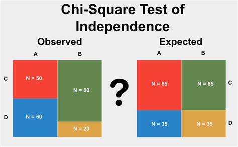
The Chi Square test is based on the concept of contingency tables, which display the frequency distribution of two categorical variables. The test calculates the difference between the observed frequencies and the expected frequencies under the null hypothesis. The null hypothesis states that there's no significant association between the two variables.
Types of Chi Square Tests
There are two types of Chi Square tests:
- Goodness-of-Fit Test: This test determines whether the observed frequencies in a single categorical variable are significantly different from the expected frequencies under a specified distribution.
- Test of Independence: This test determines whether there's a significant association between two categorical variables.
How to Perform a Chi Square Test in Excel

Performing a Chi Square test in Excel is a straightforward process. Here's a step-by-step guide:
- Prepare your data: Enter your data into a contingency table format. Each row and column should represent a category of the two variables you're testing.
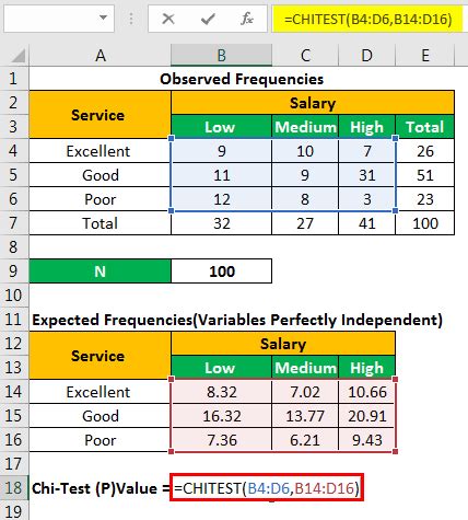
- Calculate the expected frequencies: Use the formula (Row Total x Column Total) / Grand Total to calculate the expected frequencies for each cell.
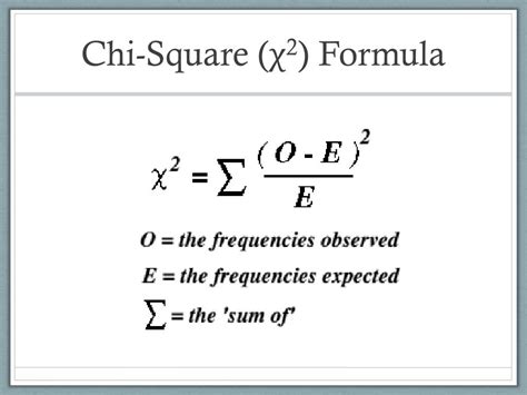
- Calculate the Chi Square statistic: Use the formula Σ [(Observed Frequency - Expected Frequency)^2 / Expected Frequency] to calculate the Chi Square statistic.
- Determine the degrees of freedom: The degrees of freedom for a Chi Square test is (r-1) x (c-1), where r is the number of rows and c is the number of columns.
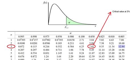
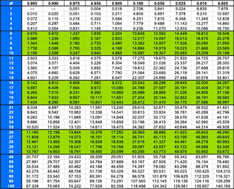
- Look up the critical value: Use a Chi Square distribution table or calculator to find the critical value for the calculated Chi Square statistic and degrees of freedom.
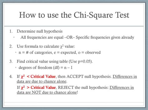
- Compare the calculated value to the critical value: If the calculated Chi Square value is greater than the critical value, reject the null hypothesis and conclude that there's a significant association between the two variables.
Using Excel Formulas to Calculate the Chi Square Statistic
You can use the following Excel formulas to calculate the Chi Square statistic:
=CHISQ.TEST(A1:E10)for a goodness-of-fit test=CHISQ.TEST(A1:E10, B1:E10)for a test of independence
Note: The CHISQ.TEST function is available in Excel 2013 and later versions.
Interpreting the Results
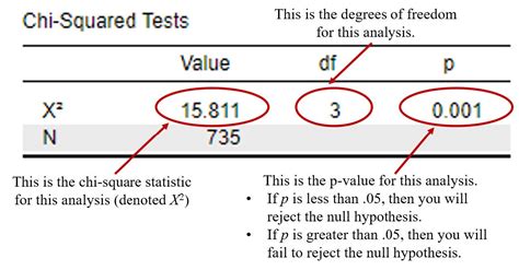
When interpreting the results of a Chi Square test, consider the following:
- P-value: The p-value represents the probability of observing the calculated Chi Square statistic under the null hypothesis. A low p-value (typically < 0.05) indicates that the observed frequencies are significantly different from the expected frequencies.
- Chi Square statistic: The Chi Square statistic represents the difference between the observed and expected frequencies. A high Chi Square statistic indicates a significant association between the two variables.
Example of a Chi Square Test in Excel
Suppose we want to determine whether there's a significant association between the color of a car (red, blue, or green) and the age of the driver (under 30, 30-50, or over 50). We can use the following contingency table:
| Age | Red | Blue | Green | Total |
|---|---|---|---|---|
| Under 30 | 10 | 15 | 20 | 45 |
| 30-50 | 20 | 30 | 15 | 65 |
| Over 50 | 15 | 10 | 5 | 30 |
| Total | 45 | 55 | 40 | 140 |
Using the CHISQ.TEST function in Excel, we calculate the Chi Square statistic and p-value:
=CHISQ.TEST(A2:C12, B2:D12) returns a p-value of 0.012
Since the p-value is less than 0.05, we reject the null hypothesis and conclude that there's a significant association between the color of the car and the age of the driver.
Gallery of Chi Square Test Images
Chi Square Test Image Gallery



Conclusion
In conclusion, the Chi Square test is a powerful statistical technique for determining whether there's a significant association between two categorical variables. By following the steps outlined in this article, you can easily perform a Chi Square test in Excel and interpret the results with confidence. Remember to always consider the limitations of the test and the assumptions that underlie it. With practice and experience, you'll become proficient in using the Chi Square test to make informed decisions in your field.
We hope this article has been helpful in your understanding of the Chi Square test. If you have any questions or comments, please feel free to share them below.
