
Creating visual representations of data in Excel can greatly enhance the understanding and analysis of that data. Adding equations to Excel graphs takes this analysis to the next level by enabling users to see the mathematical relationship between data points. This can be particularly useful in trend analysis, forecasting, and modeling. In this article, we'll walk through the process of adding equations to Excel graphs in five easy steps.
Why Add Equations to Excel Graphs?
Before diving into the steps, it's essential to understand the value of adding equations to your Excel graphs. These equations, often in the form of a trendline, help in identifying patterns, making predictions, and simplifying complex data sets. By visually representing the equation of a trendline, you can better understand the rate of change, intercepts, and other key metrics that define the relationship between variables.
Advantages of Including Equations in Excel Graphs
- Improved Data Analysis: Equations provide a clear mathematical representation of data trends.
- Forecasting: By understanding the equation behind a trend, you can extrapolate it to forecast future values.
- Simplification of Complex Data: Trendline equations help in simplifying complex data sets by highlighting the underlying pattern.
Step 1: Prepare Your Data

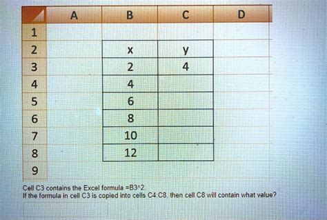
The first step in adding equations to your Excel graphs is to ensure your data is well-organized. This typically means having your data in two columns: one for the x-values (independent variable) and one for the y-values (dependent variable). Ensure the data is clean and sorted, as this will make the graphing process smoother.
Tips for Data Preparation
- Use headers for your columns.
- Sort your data by the x-variable.
- Remove any data points that are outliers or incorrect.
Step 2: Create Your Graph
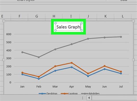
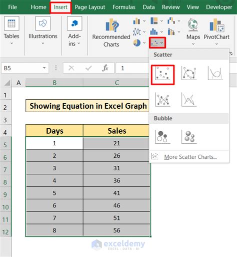
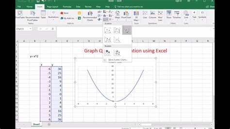
With your data prepared, you can now create a graph. To do this, select your data range (including headers), go to the "Insert" tab in the ribbon, and click on the type of graph you want to create (e.g., scatter plot). Excel will automatically generate a graph based on your data.
Choosing the Right Graph Type
- Scatter plots are ideal for showing the relationship between two variables.
- Line graphs can also be used, especially if the x-values represent a continuous time or date series.
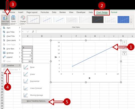
Step 3: Add a Trendline
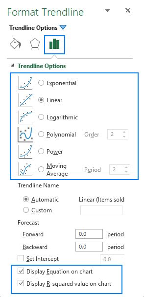
To add a trendline, click on your graph to activate the "Chart Tools" in the ribbon. Navigate to the "Analysis" section under the "Chart Tools" and click on "Trendline". Choose the type of trendline that best fits your data (linear, polynomial, etc.). Excel will calculate the best fit line for your data and display it on the graph.
Types of Trendlines
- Linear Trendline: Best for data that shows a constant rate of change.
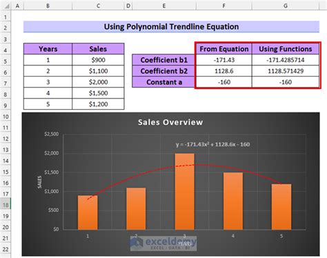
- Polynomial Trendline: Suitable for data that follows a curved pattern.
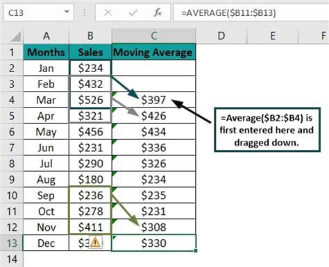
- Moving Average Trendline: Useful for smoothing out fluctuations in data over time.
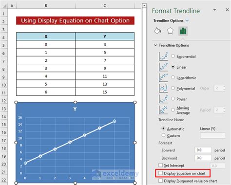
Step 4: Display the Equation
After adding a trendline, you need to display its equation. To do this, right-click on the trendline and select "Trendline Options". In the "Trendline Options" dialog box, check the box next to "Display Equation on chart". Click "OK", and the equation of the trendline will be displayed on your graph.
Tips for Displaying Equations
- Ensure the equation is visible and readable on the graph.
- You can adjust the placement and format of the equation by using the "Trendline Options" dialog box.
Step 5: Interpret and Use the Equation
The final step is to interpret and use the equation. The equation of the trendline represents the mathematical relationship between your variables. You can use this equation to make predictions, understand the rate of change, and identify key points such as intercepts.
Using Trendline Equations for Forecasting
- Substitute x-values into the equation to forecast corresponding y-values.
- Be cautious of extrapolation; the accuracy of predictions decreases as you move further away from the original data range.
Gallery of Excel Graph Equations
Excel Graph Equations

In conclusion, adding equations to Excel graphs is a powerful tool for enhancing data analysis, forecasting, and modeling. By following these five easy steps, you can unlock deeper insights into your data and make more informed decisions. Whether you're working with linear, polynomial, or moving average trendlines, displaying their equations can significantly enhance your understanding of the data.
Take the Next Step
Now that you know how to add equations to Excel graphs, take your data analysis to the next level by experimenting with different trendline types and interpreting their equations. Share your experiences, tips, or questions in the comments below.