5 Ways To Change Axis Values In Excel

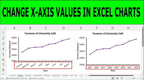
Being able to manipulate and customize data in Excel is an essential skill for any user. One common task that many users need to perform is changing the axis values in a chart. Whether you're working with a simple bar chart or a complex financial model, being able to adjust the axis values can help to clarify your data and make it more meaningful. In this article, we'll explore five different ways to change axis values in Excel, from the basics to more advanced techniques.

Method 1: Changing Axis Values through the Chart Options

The most straightforward way to change axis values in Excel is through the chart options. To do this, follow these steps:

1. Select the chart that you want to modify.
2. Click on the "Chart Options" button in the top right corner of the chart.
3. In the "Chart Options" dialog box, select the "Axes" tab.
4. In the "Axes" tab, you can adjust the minimum and maximum values for the x-axis and y-axis.
5. You can also adjust the major and minor tick marks, as well as the tick label spacing.

Using the "Axes" Tab to Customize Axis Values

The "Axes" tab in the "Chart Options" dialog box provides a range of options for customizing the axis values. You can adjust the minimum and maximum values for the x-axis and y-axis, as well as the major and minor tick marks. You can also adjust the tick label spacing to make the chart more readable.

Method 2: Changing Axis Values through the Chart Select Data Source

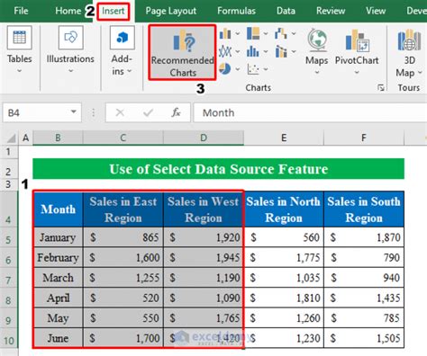
Another way to change axis values in Excel is through the "Chart Select Data Source" dialog box. To do this, follow these steps:

1. Select the chart that you want to modify.
2. Click on the "Select Data Source" button in the top right corner of the chart.
3. In the "Chart Select Data Source" dialog box, select the "Series" tab.
4. In the "Series" tab, you can adjust the axis values for each series in the chart.
5. You can also adjust the data range for each series.

Using the "Series" Tab to Customize Axis Values

The "Series" tab in the "Chart Select Data Source" dialog box provides options for customizing the axis values for each series in the chart. You can adjust the axis values, as well as the data range for each series. This can be useful if you need to compare different series in the chart.

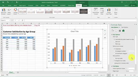
Method 3: Changing Axis Values through the Format Axis Task Pane

Excel 2013 and later versions provide a "Format Axis" task pane that makes it easy to customize the axis values. To access the "Format Axis" task pane, follow these steps:

1. Select the chart that you want to modify.
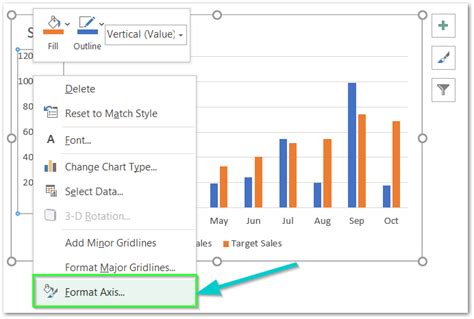
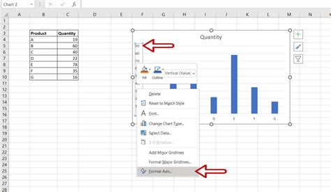
2. Select the axis that you want to customize.
3. Right-click on the axis and select "Format Axis".
4. In the "Format Axis" task pane, you can adjust the axis values, as well as the major and minor tick marks.

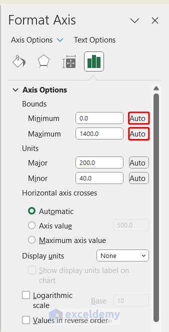
Using the "Format Axis" Task Pane to Customize Axis Values

The "Format Axis" task pane provides options for customizing the axis values, as well as the major and minor tick marks. You can adjust the minimum and maximum values for the axis, as well as the tick label spacing.

Method 4: Changing Axis Values through VBA

For more advanced users, you can use VBA (Visual Basic for Applications) to change the axis values in Excel. To do this, follow these steps:

1. Open the Visual Basic Editor by pressing "Alt + F11" or by navigating to "Developer" > "Visual Basic".
2. In the Visual Basic Editor, select the "Insert" > "Module" to insert a new module.
3. In the module, write the VBA code to change the axis values.

Example VBA Code to Change Axis Values

Here is an example of VBA code that changes the axis values:

Sub ChangeAxisValues()
    Dim cht As Chart
    Set cht = ActiveSheet.ChartObjects(1).Chart
    cht.Axes(xlCategory).MinimumScale = 10
    cht.Axes(xlCategory).MaximumScale = 20
End Sub

This code changes the minimum and maximum values for the x-axis in the first chart in the active worksheet.

Method 5: Changing Axis Values through Power Query

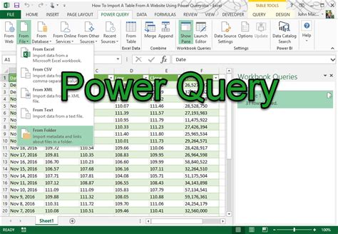
Power Query is a powerful tool in Excel that allows you to manipulate and transform data. You can use Power Query to change the axis values in a chart. To do this, follow these steps:

1. Open the Power Query Editor by navigating to "Data" > "New Query" > "From Other Sources" > "Blank Query".
2. In the Power Query Editor, select the data range that you want to use for the chart.
3. Use the "Add Column" and "Transform" tabs to manipulate the data and change the axis values.

Using Power Query to Customize Axis Values

Power Query provides a range of options for customizing the axis values. You can use the "Add Column" and "Transform" tabs to manipulate the data and change the axis values. This can be useful if you need to transform the data before creating the chart.

Excel Axis Values Gallery

We hope that this article has provided you with a comprehensive guide to changing axis values in Excel. Whether you're using the chart options, select data source, format axis task pane, VBA, or Power Query, there are many ways to customize the axis values in Excel. By following the steps outlined in this article, you should be able to change the axis values in your chart and make it more meaningful and effective.

If you have any questions or need further assistance, please don't hesitate to ask. You can also share your own tips and tricks for changing axis values in the comments below.