Compare Columns In Excel To Find Matches Easily

Comparing columns in Excel is a common task that can be daunting, especially when dealing with large datasets. Fortunately, Excel provides several methods to make this process easier and more efficient. In this article, we will explore the different ways to compare columns in Excel to find matches easily.

Why Compare Columns in Excel?

Comparing columns in Excel is essential in various scenarios, such as:

• Identifying duplicates or matching values between two lists
• Verifying data accuracy by comparing values in two columns
• Finding missing or mismatched data between two datasets
• Consolidating data from multiple sources

Method 1: Using the VLOOKUP Function

The VLOOKUP function is a popular method for comparing columns in Excel. It allows you to search for a value in a table and return a corresponding value from another column.

Syntax: VLOOKUP(lookup_value, table_array, col_index_num, [range_lookup])

• Lookup_value: the value to search for
• Table_array: the range of cells that contains the data to search
• Col_index_num: the column number that contains the value to return
• Range_lookup: [optional] a logical value that specifies whether to perform an exact or approximate match

Example: =VLOOKUP(A2, B:C, 2, FALSE)

This formula searches for the value in cell A2 in the first column of the range B:C and returns the corresponding value in the second column.

Method 1.1: Using INDEX-MATCH Functions

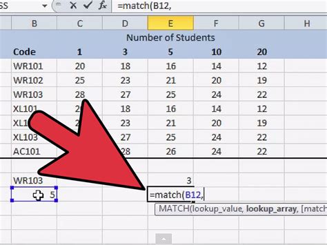
The INDEX-MATCH function combination is a more flexible and powerful alternative to VLOOKUP.

Syntax: INDEX(range, MATCH(lookup_value, range, [match_type]))

• Range: the range of cells that contains the data to search
• Lookup_value: the value to search for
• Match_type: [optional] a value that specifies the type of match to perform

Example: =INDEX(C:C, MATCH(A2, B:B, 0))

This formula searches for the value in cell A2 in the range B:B and returns the corresponding value in the range C:C.

Method 2: Using Conditional Formatting

Conditional formatting is a feature in Excel that allows you to highlight cells based on specific conditions.

Example:

1. Select the range of cells to compare (e.g., A1:A10 and B1:B10)
2. Go to Home > Conditional Formatting > New Rule
3. Select "Use a formula to determine which cells to format"
4. Enter the formula: =A1=B1
5. Click "Format" and select a fill color
6. Click "OK"

This will highlight the cells in column A that match the corresponding cells in column B.

Method 2.1: Using Formula-Based Conditional Formatting

You can also use a formula-based approach to conditional formatting.

Example:

1. Select the range of cells to compare (e.g., A1:A10 and B1:B10)
2. Go to Home > Conditional Formatting > New Rule
3. Select "Use a formula to determine which cells to format"
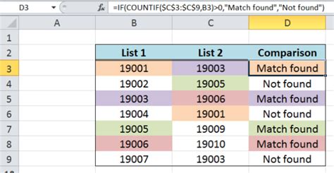
4. Enter the formula: =COUNTIF(B:B, A1)>0
5. Click "Format" and select a fill color
6. Click "OK"

This will highlight the cells in column A that have a match in column B.

Method 3: Using Power Query

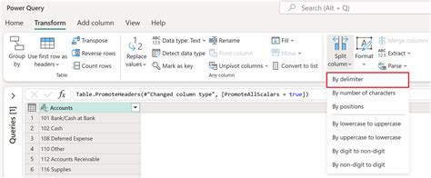
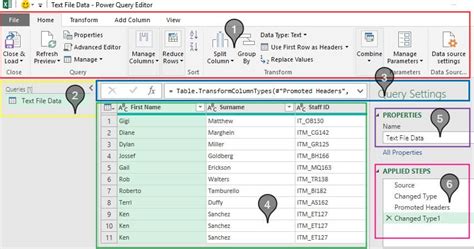
Power Query is a powerful data manipulation tool in Excel that allows you to compare columns and perform data matching.

Example:

1. Go to Data > New Query > From Other Sources > Blank Query
2. Enter the formula: = Table.Join(Table1, Table2, {"Column1"}, {"Column2"}, JoinKind.Inner)
3. Click "OK"

This will create a new table that contains the matched data from the two tables.

Method 3.1: Using Power Query's Merge Queries Feature

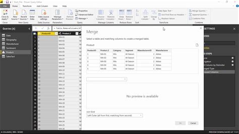
Power Query also provides a Merge Queries feature that allows you to compare columns and perform data matching.

Example:

1. Go to Data > New Query > From Other Sources > Blank Query
2. Enter the formula: = Table.Merge(Table1, Table2, {"Column1"}, {"Column2"}, JoinKind.Inner)
3. Click "OK"

This will create a new table that contains the matched data from the two tables.

Gallery of Excel Column Comparison

Excel Column Comparison Gallery

We hope this article has helped you learn how to compare columns in Excel to find matches easily. Whether you use the VLOOKUP function, conditional formatting, or Power Query, there are many methods to choose from. Remember to explore each method in more detail and practice using them to become proficient in comparing columns in Excel.

Share your thoughts: Have you used any of these methods to compare columns in Excel? Do you have any tips or tricks to share? Leave a comment below and let's start a conversation!