5 Ways To Compare Columns In Google Sheets

Comparing columns in Google Sheets is a crucial task for data analysis, research, and decision-making. Whether you're working with financial data, customer information, or scientific research, being able to compare columns efficiently is essential. Google Sheets offers several ways to compare columns, each with its own strengths and uses. In this article, we'll explore five methods to compare columns in Google Sheets, along with practical examples and step-by-step instructions.

1. Using the =A1=B1 Formula

The most straightforward way to compare two columns in Google Sheets is by using a simple formula. This method is useful for comparing small datasets or when you need to compare individual cells.

To compare two columns using the =A1=B1 formula:

• Select the cell where you want to display the comparison result.
• Type the formula =A1=B1, assuming you want to compare the values in cells A1 and B1.
• Press Enter to apply the formula.
• The formula will return TRUE if the values are identical and FALSE otherwise.
• To compare entire columns, copy the formula down to the other cells in the column.

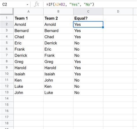
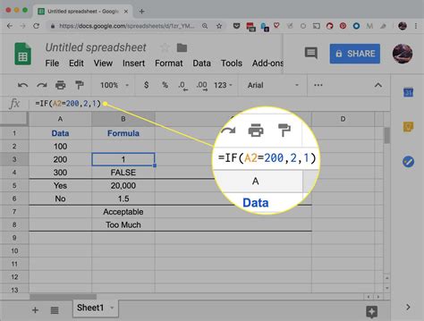
2. Using the IF Function

The IF function in Google Sheets allows you to compare columns and perform actions based on the comparison result. This method is useful for more complex comparisons, such as comparing multiple columns or performing calculations based on the comparison result.

To compare two columns using the IF function:

• Select the cell where you want to display the comparison result.
• Type the formula =IF(A1=B1, "Match", "No Match"), assuming you want to compare the values in cells A1 and B1 and display "Match" if they are identical and "No Match" otherwise.
• Press Enter to apply the formula.
• The formula will return "Match" if the values are identical and "No Match" otherwise.
• To compare entire columns, copy the formula down to the other cells in the column.

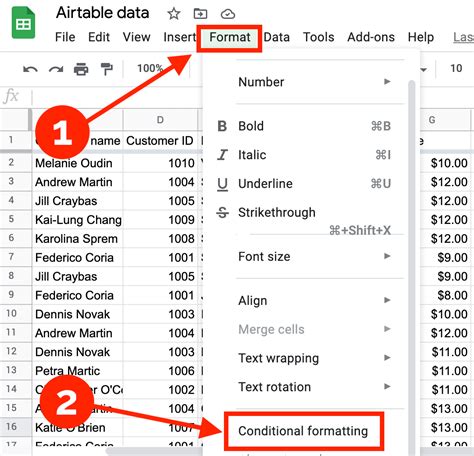
3. Using Conditional Formatting

Conditional formatting in Google Sheets allows you to highlight cells based on specific conditions, including comparisons between columns. This method is useful for visualizing the comparison result and identifying patterns in your data.

To compare two columns using conditional formatting:

• Select the range of cells you want to format.
• Go to the "Format" tab in the top menu.
• Select "Conditional formatting."
• In the "Format cells if" dropdown menu, select "Custom formula is."
• Type the formula =A1=B1, assuming you want to compare the values in cells A1 and B1.
• Choose a formatting style, such as a background color or font color.
• Click "Done" to apply the formatting.
• The cells that meet the comparison condition will be formatted accordingly.

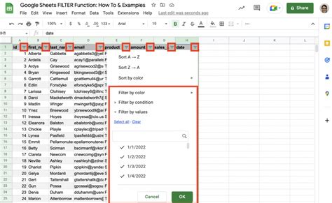
4. Using the FILTER Function

The FILTER function in Google Sheets allows you to filter data based on specific conditions, including comparisons between columns. This method is useful for extracting specific data from your spreadsheet and performing calculations on the filtered data.

To compare two columns using the FILTER function:

• Select the cell where you want to display the filtered data.
• Type the formula =FILTER(A:B, A:A=B:B), assuming you want to filter the data in columns A and B based on the comparison between the two columns.
• Press Enter to apply the formula.
• The formula will return the filtered data.
• To perform calculations on the filtered data, use the SUM, AVERAGE, or other functions.

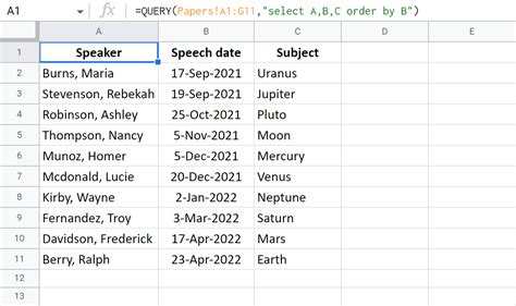
5. Using the QUERY Function

The QUERY function in Google Sheets allows you to perform SQL-like queries on your data, including comparisons between columns. This method is useful for complex data analysis and data visualization.

To compare two columns using the QUERY function:

• Select the cell where you want to display the query result.
• Type the formula =QUERY(A:B, "SELECT * WHERE A = B"), assuming you want to compare the values in columns A and B and display the rows where the values are identical.
• Press Enter to apply the formula.
• The formula will return the query result.
• To perform calculations on the query result, use the SUM, AVERAGE, or other functions.

Google Sheets Image Gallery

We hope this article has helped you learn how to compare columns in Google Sheets using various methods. Whether you're working with small datasets or large datasets, Google Sheets offers a range of tools and functions to help you compare columns efficiently and effectively. By mastering these methods, you'll be able to make more informed decisions, identify patterns in your data, and create more accurate reports.

If you have any questions or need further assistance, please don't hesitate to ask. Share your experiences and tips for comparing columns in Google Sheets in the comments below.