The Chi-Square test is a widely used statistical method for determining whether there is a significant association between two categorical variables. Excel provides a simple and efficient way to perform the Chi-Square test, making it easier for researchers and analysts to analyze their data. In this article, we will guide you through the 5 steps to perform a Chi-Square test in Excel.

Step 1: Prepare Your Data
Before performing the Chi-Square test, it is essential to prepare your data. The test requires two categorical variables, which should be organized in a contingency table. A contingency table is a table that displays the frequency distribution of two or more variables.
To prepare your data, follow these steps:
- Organize your data in a table with two variables (e.g., variable A and variable B).
- Ensure that each variable has two or more categories.
- Count the frequency of each combination of categories.
For example, let's say we want to determine whether there is a significant association between the gender of a person and their preference for a particular brand of soda. Our data might look like this:
| Gender | Soda Preference |
|---|---|
| Male | Coke |
| Male | Pepsi |
| Female | Coke |
| Female | Pepsi |

Step 2: Create a Contingency Table
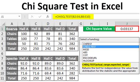
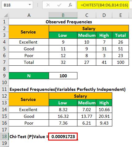
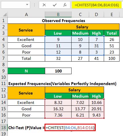
Once you have prepared your data, create a contingency table using the frequency counts. The table should have rows representing the categories of one variable and columns representing the categories of the other variable.
Using our example, the contingency table might look like this:
| Coke | Pepsi | Total | |
|---|---|---|---|
| Male | 20 | 30 | 50 |
| Female | 15 | 25 | 40 |
| Total | 35 | 55 | 90 |

Step 3: Calculate the Expected Frequencies
The next step is to calculate the expected frequencies under the assumption of no association between the two variables. The expected frequencies can be calculated using the formula:
Expected frequency = (Row total x Column total) / Total
Using our example, the expected frequencies might look like this:
| Coke | Pepsi | Total | |
|---|---|---|---|
| Male | 19.44 | 30.56 | 50 |
| Female | 15.56 | 24.44 | 40 |
| Total | 35 | 55 | 90 |

Step 4: Calculate the Chi-Square Statistic
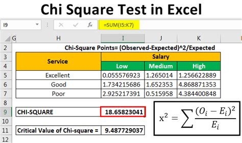
The Chi-Square statistic is calculated using the formula:
Chi-Square = Σ [(Observed frequency - Expected frequency)^2 / Expected frequency]
Using our example, the Chi-Square statistic might be:
Chi-Square = [(20-19.44)^2 / 19.44] + [(30-30.56)^2 / 30.56] + [(15-15.56)^2 / 15.56] + [(25-24.44)^2 / 24.44] = 0.058 + 0.006 + 0.058 + 0.044 = 0.166

Step 5: Determine the Significance
The final step is to determine the significance of the Chi-Square statistic. This can be done using a Chi-Square distribution table or by calculating the p-value.
Using our example, let's say we have a significance level of 0.05. If the p-value is less than 0.05, we reject the null hypothesis and conclude that there is a significant association between the two variables.

Chi Square Test Image Gallery


In conclusion, performing a Chi-Square test in Excel is a straightforward process that can help you determine whether there is a significant association between two categorical variables. By following these 5 steps, you can easily perform a Chi-Square test and make informed decisions based on your data.
