
Creating a chart in Excel for Mac is a straightforward process that can help you to effectively communicate data insights and trends to your audience. Whether you're a student, professional, or simply looking to organize your personal data, learning how to create a chart in Excel can be a valuable skill. In this article, we'll walk you through the 5 easy steps to create a chart in Excel for Mac.
Understanding the Benefits of Using Charts in Excel

Before we dive into the steps, let's quickly discuss the benefits of using charts in Excel. Charts can help to:
- Simplify complex data
- Identify trends and patterns
- Enhance data visualization
- Communicate insights more effectively
- Support data-driven decision making
Step 1: Prepare Your Data

The first step in creating a chart in Excel is to prepare your data. This involves ensuring that your data is organized in a way that can be easily interpreted by Excel. Here are some tips to keep in mind:
- Use a header row to label your columns
- Ensure that each column has a consistent data type (e.g., all numbers or all text)
- Use separate columns for each data series
- Remove any unnecessary data or formatting
Example: Preparing Sales Data for a Chart
| Month | Sales |
|---|---|
| January | 1000 |
| February | 1200 |
| March | 1500 |
| April | 1800 |
| May | 2000 |
Step 2: Select Your Data
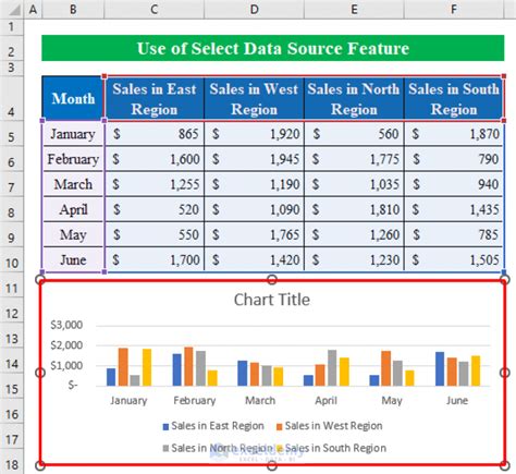
Once your data is prepared, select the entire data range that you want to include in your chart. To do this, simply click and drag your mouse to highlight the data range.
Example: Selecting the Sales Data Range
| Month | Sales |
|---|---|
| January | 1000 |
| February | 1200 |
| March | 1500 |
| April | 1800 |
| May | 2000 |
Step 3: Choose a Chart Type

With your data selected, it's time to choose a chart type. Excel offers a variety of chart types, including column charts, line charts, pie charts, and more. To choose a chart type, go to the "Insert" tab and click on the "Chart" button.
Example: Choosing a Column Chart
- Click on the "Insert" tab
- Click on the "Chart" button
- Select "Column Chart" from the drop-down menu
Step 4: Customize Your Chart

Once you've chosen a chart type, you can customize your chart to suit your needs. This includes adding titles, labels, and legends, as well as modifying the chart's appearance and layout.
Example: Customizing a Column Chart
- Add a chart title: "Monthly Sales"
- Add axis labels: "Month" and "Sales"
- Add a legend: "Sales Data"
- Change the chart colors: select a color scheme that matches your brand or preferences
Step 5: Finalize and Refine Your Chart
The final step is to finalize and refine your chart. This includes checking for errors, ensuring that the chart is properly formatted, and making any final adjustments.
Example: Finalizing a Column Chart
- Check for errors: ensure that the data is accurate and the chart is properly formatted
- Make final adjustments: adjust the chart size, layout, and appearance as needed
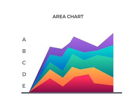
Excel Chart Gallery


We hope this article has helped you to learn how to create a chart in Excel for Mac. With these 5 easy steps, you can create a variety of charts to help you to communicate data insights and trends to your audience. Remember to practice, experiment, and refine your chart-creating skills to become an Excel expert!