
Using the MATCH function in Excel can be a powerful way to perform lookups and find the relative position of a value within a range. However, sometimes you may need to nest the MATCH function with other functions to achieve more complex tasks. In this article, we will explore five ways to nest a MATCH function in Excel.
Why Nest the MATCH Function?
Before we dive into the different ways to nest the MATCH function, let's understand why you might need to do so. The MATCH function returns the relative position of a value within a range, but it doesn't return the actual value. By nesting the MATCH function with other functions, you can perform more complex lookups and return the actual value or perform calculations based on the result.
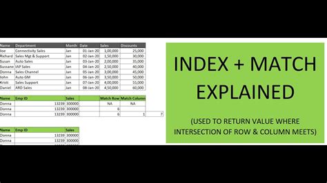
Method 1: Nesting MATCH with INDEX
One of the most common ways to nest the MATCH function is with the INDEX function. The INDEX function returns a value at a specified position within a range, and when combined with the MATCH function, it can perform lookups and return the actual value.
Formula: =INDEX(range, MATCH(lookup_value, lookup_array, [match_type])
For example, suppose you have a range of names in column A and a range of corresponding ages in column B. You can use the following formula to return the age of a specific person:
=INDEX(B:B, MATCH("John", A:A, 0))
This formula returns the age of John by finding the relative position of John in the range of names and using that position to return the corresponding age.
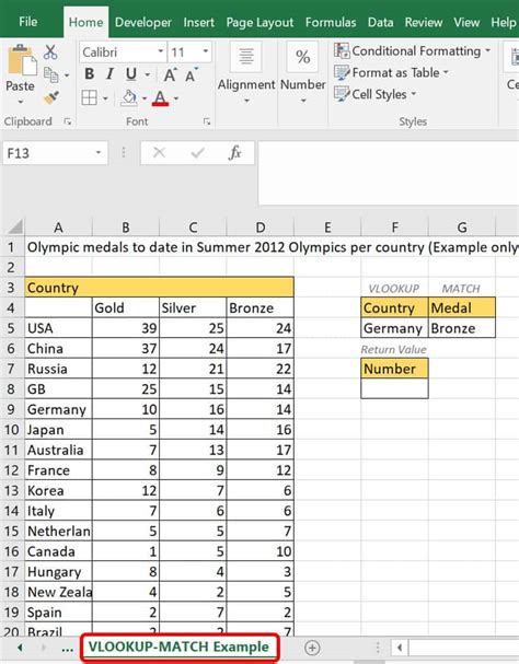
Method 2: Nesting MATCH with VLOOKUP
Another way to nest the MATCH function is with the VLOOKUP function. The VLOOKUP function performs a vertical lookup and returns a value from a table based on a lookup value. By combining VLOOKUP with the MATCH function, you can perform more complex lookups and return the actual value.
Formula: =VLOOKUP(lookup_value, table_array, MATCH(lookup_value, table_array, [match_type]), [range_lookup])
For example, suppose you have a table with names in column A and ages in column B. You can use the following formula to return the age of a specific person:
=VLOOKUP("John", A:B, MATCH("John", A:A, 0), FALSE)
This formula returns the age of John by finding the relative position of John in the range of names and using that position to return the corresponding age.
Method 3: Nesting MATCH with IFERROR
The IFERROR function returns a value if an error occurs, and when combined with the MATCH function, it can handle errors that may occur during the lookup process.
Formula: =IFERROR(MATCH(lookup_value, lookup_array, [match_type]), error_value)
For example, suppose you have a range of names in column A and you want to find the relative position of a specific name. If the name is not found, you can return a custom error message.
=IFERROR(MATCH("John", A:A, 0), "Name not found")
This formula returns the relative position of John in the range of names, and if John is not found, it returns the error message "Name not found".

Method 4: Nesting MATCH with IF
The IF function tests a condition and returns one value if true and another value if false. By combining the IF function with the MATCH function, you can perform conditional lookups and return different values based on the result.
Formula: =IF(MATCH(lookup_value, lookup_array, [match_type])>0, value_if_true, value_if_false)
For example, suppose you have a range of names in column A and you want to find the relative position of a specific name. If the name is found, you can return a custom message.
=IF(MATCH("John", A:A, 0)>0, "Name found", "Name not found")
This formula returns the message "Name found" if John is found in the range of names, and "Name not found" if John is not found.

Method 5: Nesting MATCH with CHOOSE
The CHOOSE function returns a value from a list based on a position, and when combined with the MATCH function, it can perform lookups and return different values based on the result.
Formula: =CHOOSE(MATCH(lookup_value, lookup_array, [match_type]), value1, [value2],...)
For example, suppose you have a range of names in column A and a range of corresponding colors in column B. You can use the following formula to return the color of a specific person:
=CHOOSE(MATCH("John", A:A, 0), "Red", "Blue", "Green")
This formula returns the color of John by finding the relative position of John in the range of names and using that position to return the corresponding color.
Gallery of Nesting MATCH Function Examples
Nesting MATCH Function Examples


Final Thoughts
Nesting the MATCH function with other functions can help you perform more complex lookups and return the actual value or perform calculations based on the result. By using the methods outlined in this article, you can take your Excel skills to the next level and perform tasks that would be difficult or impossible to achieve with a single function. Do you have any questions about nesting the MATCH function? Share your thoughts and examples in the comments below!