3 Ways To Plot Min, Max, And Average In Excel

How to Plot Min, Max, and Average in Excel

Working with data in Excel can be a challenge, especially when it comes to visualizing and understanding the data. One common requirement is to plot the minimum, maximum, and average values of a dataset. This can be achieved using Excel's built-in charting features and formulas. In this article, we will explore three ways to plot min, max, and average in Excel, making it easier to analyze and understand your data.

Method 1: Using Formulas and a Line Chart

The first method involves using formulas to calculate the minimum, maximum, and average values of your dataset, and then creating a line chart to visualize the data. Here's how:

• Calculate the minimum value using the MIN function: =MIN(range)
• Calculate the maximum value using the MAX function: =MAX(range)
• Calculate the average value using the AVERAGE function: =AVERAGE(range)
• Create a new table with the calculated values
• Select the data range and go to the "Insert" tab in the ribbon
• Click on the "Line Chart" button and select the desired chart type

This method is straightforward and easy to implement, but it requires manual updates whenever the data changes.

Method 1 Example

Suppose we have a dataset of exam scores for a class of students. We want to plot the minimum, maximum, and average scores.

Student	Score
John	85
Mary	90
David	78
Emily	92
...	...

Using the formulas, we get:

Minimum	Maximum	Average
78	92	85.5

Creating a line chart with these values gives us a clear visualization of the data.

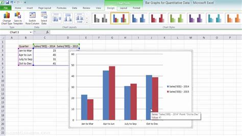
Method 2: Using a PivotTable and a Bar Chart

The second method involves using a PivotTable to summarize the data and then creating a bar chart to visualize the results. Here's how:

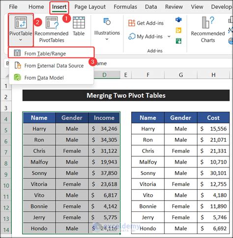
• Create a PivotTable from the dataset
• Drag the field you want to analyze to the "Values" area
• Right-click on the field and select "Value Field Settings"
• In the "Value Field Settings" dialog box, select "Min", "Max", and "Average" as the value fields
• Create a new bar chart using the PivotTable data

This method is more dynamic than the first method, as the PivotTable will automatically update when the data changes.

Method 2 Example

Using the same dataset as before, we create a PivotTable and drag the "Score" field to the "Values" area. We then select "Min", "Max", and "Average" as the value fields.

Minimum	Maximum	Average
78	92	85.5

Creating a bar chart with these values gives us a clear visualization of the data.

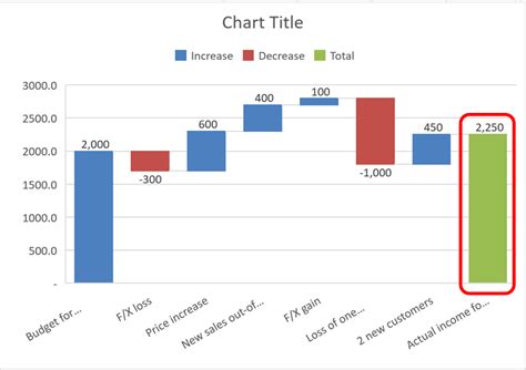
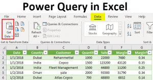
Method 3: Using Power Query and a Waterfall Chart

The third method involves using Power Query to summarize the data and then creating a waterfall chart to visualize the results. Here's how:

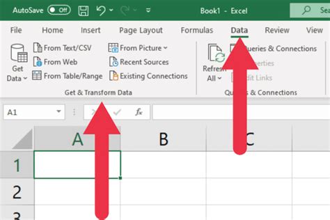
• Go to the "Data" tab in the ribbon and select "New Query"
• Connect to the dataset and load it into Power Query
• Use the "Group By" function to group the data by the desired field
• Use the "Aggregate" function to calculate the minimum, maximum, and average values
• Create a new waterfall chart using the Power Query data

This method is more powerful than the first two methods, as Power Query allows for more complex data analysis and manipulation.

Method 3 Example

Using the same dataset as before, we create a new query and load the data into Power Query. We then use the "Group By" function to group the data by the "Student" field and the "Aggregate" function to calculate the minimum, maximum, and average scores.

Student	Minimum	Maximum	Average
John	85	85	85
Mary	90	90	90
David	78	78	78
Emily	92	92	92
...	...	...	...

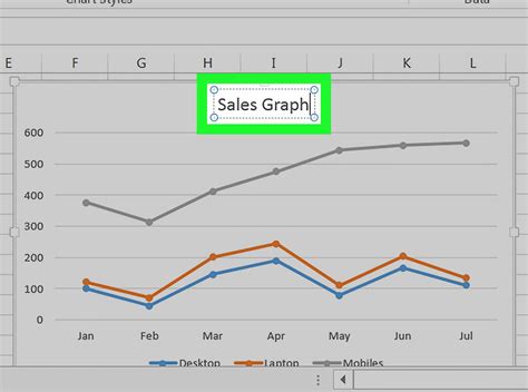
Creating a waterfall chart with these values gives us a clear visualization of the data.

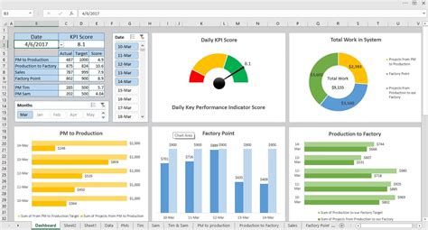
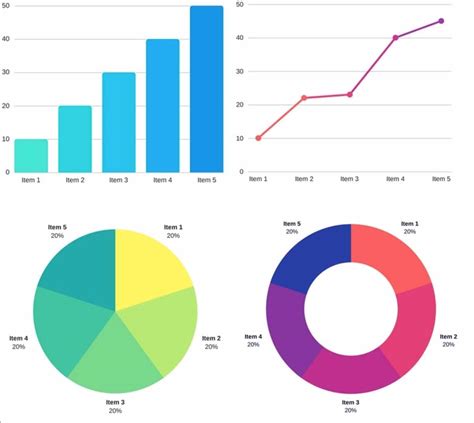
Excel Chart Examples

In conclusion, plotting min, max, and average values in Excel can be achieved using various methods, each with its own strengths and weaknesses. By choosing the right method for your data and analysis needs, you can create informative and engaging charts that help you better understand your data.