Using the IFERROR function in conjunction with VLOOKUP in Excel can significantly enhance your data analysis and management capabilities. The VLOOKUP function is a powerful tool for searching and retrieving data from a table, but it can be prone to errors, especially if the value being searched for is not found. This is where the IFERROR function comes into play, allowing you to manage and handle errors more elegantly. Here, we will explore five practical ways to use IFERROR with VLOOKUP in Excel, ensuring that your data analysis remains robust and error-free.
Understanding IFERROR and VLOOKUP
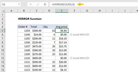
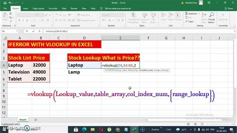
Before diving into the practical applications, let's briefly understand the functions we are working with. The VLOOKUP function searches for a value in the first column of a table array and returns a value in the same row from another column that you specify. The IFERROR function, on the other hand, returns a value you specify if a formula evaluates to an error; otherwise, it returns the result of the formula.
Basic Syntax
VLOOKUP(lookup_value, table_array, col_index_num, [range_lookup])IFERROR(cell, value_if_error)
Method 1: Handling Missing Values

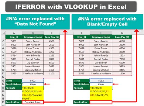
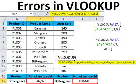
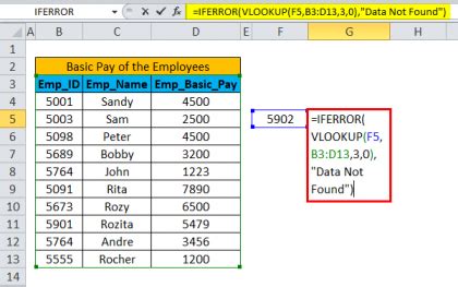
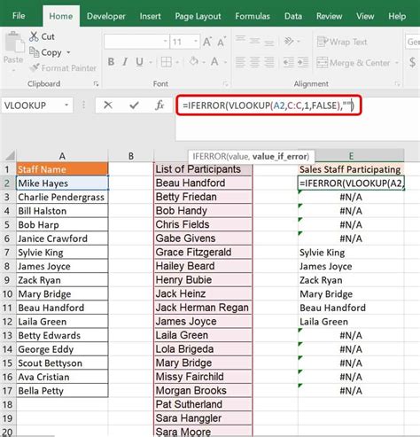
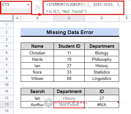
One of the most common issues with VLOOKUP is handling missing values. If the value you're searching for doesn't exist in the first column of your table array, VLOOKUP returns a #N/A error. By wrapping VLOOKUP in IFERROR, you can specify a return value when this occurs, making your spreadsheet more user-friendly.
=IFERROR(VLOOKUP(A2, B:C, 2, FALSE), "Not Found")
In this example, if the value in cell A2 is not found in the first column of the range B:C, the formula will return "Not Found" instead of #N/A.
Method 2: Returning a Default Value

Sometimes, you might want to return a default value if the VLOOKUP returns an error. This could be useful in scenarios where you want to maintain a uniform output, even if the data is missing.
=IFERROR(VLOOKUP(A2, B:C, 2, FALSE), 0)
In this case, if the VLOOKUP fails to find the value, it will return 0 instead of an error message.
Method 3: Providing a Custom Error Message
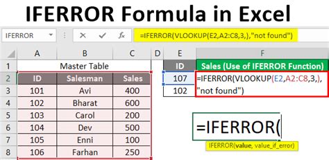
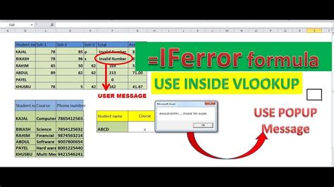
You can tailor the error message to provide more context or instructions for the user. This can be particularly useful in shared workbooks or when you're distributing templates.
=IFERROR(VLOOKUP(A2, B:C, 2, FALSE), "Please check the input value or ensure it exists in the database.")
This approach not only handles the error but also guides the user on what to do next.
Method 4: Combining with Other Functions
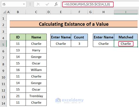
The beauty of Excel lies in its flexibility and the ability to combine functions to achieve complex calculations. You can nest IFERROR with other functions like IF, INDEX/MATCH, or even another VLOOKUP to create powerful formulas.
=IFERROR(IF(VLOOKUP(A2, B:C, 2, FALSE)>10, "High", "Low"), "Invalid Input")
In this example, the formula checks if the result of the VLOOKUP is greater than 10 and returns "High" or "Low" accordingly. If the VLOOKUP returns an error, it catches it and returns "Invalid Input".
Method 5: Using IFERROR with Multiple VLOOKUPs
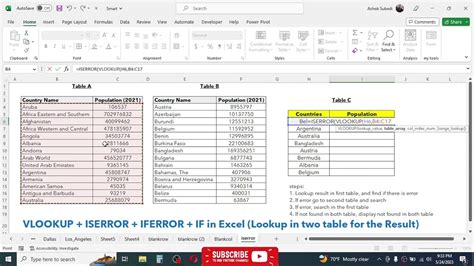
In scenarios where you need to search across multiple tables or ranges, you might end up with multiple VLOOKUPs. IFERROR can be used to handle errors for each of these VLOOKUPs, ensuring that your formula remains robust.
=IFERROR(VLOOKUP(A2, B:C, 2, FALSE), IFERROR(VLOOKUP(A2, D:E, 2, FALSE), "Not Found in Either Database"))
This formula searches for the value in two different ranges and returns "Not Found in Either Database" if it's not found in either.
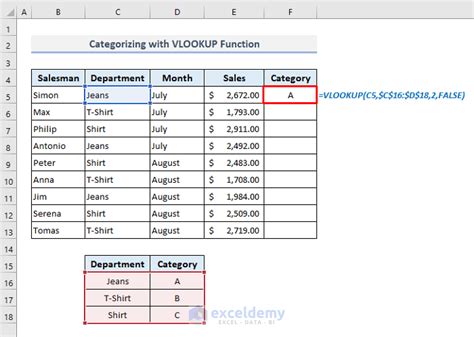
Gallery of IFERROR and VLOOKUP Examples
IFERROR and VLOOKUP Examples

Final Thoughts
Utilizing IFERROR in conjunction with VLOOKUP can significantly enhance the robustness and user-friendliness of your Excel spreadsheets. By understanding and applying the methods outlined above, you can create more reliable and efficient data management systems. Whether you're handling missing values, returning default values, or providing custom error messages, the combination of IFERROR and VLOOKUP is a powerful tool in your Excel arsenal.
We hope this comprehensive guide has not only educated you on the how-to aspects but has also inspired you to explore further applications of these functions in your day-to-day Excel usage. As always, practice is key, so don't hesitate to experiment and find new ways to leverage these functions to solve complex data challenges.
