Excel Mapping Values Made Easy With Simple Formulas

The world of Excel can be overwhelming, especially when it comes to mapping values. Whether you're a beginner or an advanced user, mapping values is an essential skill to master. In this article, we'll explore the basics of Excel mapping values and provide simple formulas to make the process easier.

Understanding Mapping Values in Excel

Mapping values in Excel is the process of matching data from one table or range to another based on a common key. This technique is useful when you need to combine data from multiple sources or update data in one table based on changes in another. In this article, we'll focus on using simple formulas to map values in Excel.

The Benefits of Mapping Values in Excel

Mapping values in Excel offers several benefits, including:

• Improved data accuracy and consistency
• Reduced data entry errors
• Enhanced data analysis and reporting capabilities
• Increased productivity and efficiency

Using VLOOKUP to Map Values in Excel

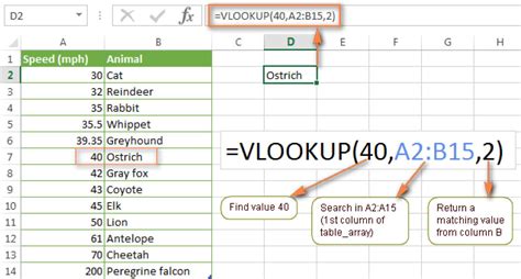
One of the most common formulas used for mapping values in Excel is the VLOOKUP function. The VLOOKUP function searches for a value in a table or range and returns a corresponding value from another column.

The syntax for the VLOOKUP function is:

VLOOKUP(lookup_value, table_array, col_index_num, [range_lookup])

Where:

• lookup_value is the value you want to search for
• table_array is the range of cells that contains the data you want to search
• col_index_num is the column number that contains the value you want to return
• [range_lookup] is an optional argument that specifies whether you want an exact match or an approximate match

For example, suppose you have a table with the following data:

Employee ID	Name	Department
101	John Smith	Sales
102	Jane Doe	Marketing
103	Bob Johnson	IT

You can use the VLOOKUP function to retrieve the department for a given employee ID.

=VLOOKUP(101, A:C, 3, FALSE)

This formula searches for the value 101 in the first column of the range A:C and returns the value in the third column (Department).

Using INDEX-MATCH to Map Values in Excel

Another powerful formula for mapping values in Excel is the INDEX-MATCH function combination. This formula is more flexible and powerful than VLOOKUP, especially when working with large datasets.

The syntax for the INDEX-MATCH function combination is:

INDEX(range, MATCH(lookup_value, lookup_array, [match_type])

Where:

• range is the range of cells that contains the data you want to return
• lookup_value is the value you want to search for
• lookup_array is the range of cells that contains the data you want to search
• [match_type] is an optional argument that specifies the type of match you want to perform

For example, suppose you have the same table as before:

Employee ID	Name	Department
101	John Smith	Sales
102	Jane Doe	Marketing
103	Bob Johnson	IT

You can use the INDEX-MATCH function combination to retrieve the department for a given employee ID.

=INDEX(C:C, MATCH(101, A:A, 0))

This formula searches for the value 101 in the first column of the range A:A and returns the value in the third column (Department).

Using Power Query to Map Values in Excel

Power Query is a powerful tool in Excel that allows you to easily map values from one table to another. With Power Query, you can perform complex data transformations and mappings with ease.

To use Power Query to map values, follow these steps:

1. Go to the Data tab in the ribbon and click on New Query.
2. Select From Other Sources and then select Blank Query.
3. In the Query Editor, click on Add Column and then select Merge Queries.
4. Select the two tables you want to merge and specify the common key.
5. Click on OK to merge the tables.

For example, suppose you have two tables:

Table 1

Employee ID	Name
101	John Smith
102	Jane Doe
103	Bob Johnson

Table 2

Employee ID	Department
101	Sales
102	Marketing
103	IT

You can use Power Query to merge the two tables based on the Employee ID column.

Best Practices for Mapping Values in Excel

Here are some best practices to keep in mind when mapping values in Excel:

• Use meaningful column names and headers to make your data easier to understand.
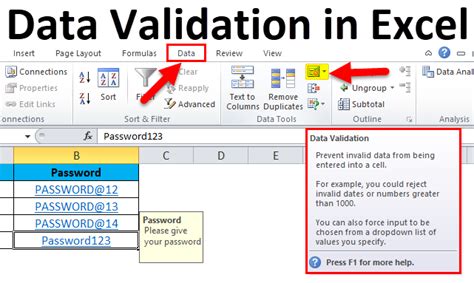
• Use data validation to ensure that your data is accurate and consistent.
• Use formatting to make your data easier to read and understand.
• Use formulas and functions to automate your data mappings.
• Test your data mappings thoroughly to ensure that they are accurate and reliable.

Excel Mapping Values Image Gallery

We hope this article has helped you understand the basics of Excel mapping values and how to use simple formulas to make the process easier. Whether you're a beginner or an advanced user, mastering the art of mapping values in Excel can save you time and improve your productivity. So, what are you waiting for? Start mapping your values today and take your Excel skills to the next level!