Matching multiple criteria in Excel can be a challenging task, especially when working with large datasets. However, there are several ways to achieve this, and we will explore five of them in this article.
The ability to match multiple criteria is essential in various Excel applications, such as data analysis, filtering, and reporting. Whether you need to identify records that meet specific conditions or extract data that satisfies multiple criteria, these methods will help you accomplish your goals efficiently.

Using the FILTER Function
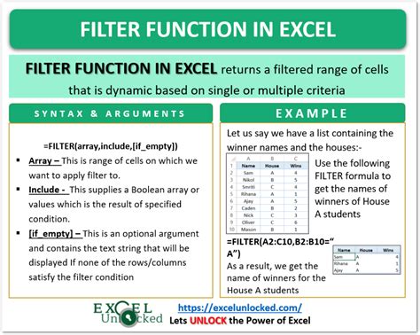
The FILTER function is one of the most straightforward methods to match multiple criteria in Excel. This function allows you to filter a range of data based on multiple conditions. The syntax for the FILTER function is:
FILTER(range, include, [if_empty])
Where:
- range is the range of cells that you want to filter
- include is the condition that you want to apply to the range
- if_empty is an optional argument that specifies what to return if the filtered range is empty
For example, suppose you have a range of data in cells A1:C10, and you want to filter the data to show only the records where the value in column A is "John" and the value in column B is "Sales".
Example Using FILTER Function
| Name | Department | Sales |
|---|---|---|
| John | Sales | 100 |
| Jane | Marketing | 200 |
| John | Sales | 300 |
| Bob | Sales | 400 |
To filter the data using the FILTER function, you can use the following formula:
=FILTER(A1:C10, (A1:A10="John") * (B1:B10="Sales"))
This formula will return only the records where the value in column A is "John" and the value in column B is "Sales".
Using the INDEX-MATCH Function Combination
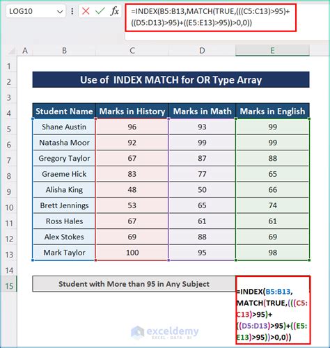
The INDEX-MATCH function combination is another powerful method to match multiple criteria in Excel. This combination allows you to look up values in a range of cells and return a corresponding value from another range.
The syntax for the INDEX-MATCH function combination is:
INDEX(range, MATCH(lookup_value, lookup_array, [match_type]))
Where:
- range is the range of cells that you want to look up
- lookup_value is the value that you want to look up
- lookup_array is the range of cells that contains the values to look up
- match_type is an optional argument that specifies the type of match to perform
For example, suppose you have a range of data in cells A1:C10, and you want to look up the sales value for a specific employee in a specific department.
Example Using INDEX-MATCH Function Combination
| Name | Department | Sales |
|---|---|---|
| John | Sales | 100 |
| Jane | Marketing | 200 |
| John | Sales | 300 |
| Bob | Sales | 400 |
To look up the sales value using the INDEX-MATCH function combination, you can use the following formula:
=INDEX(C:C, MATCH(1, (A:A="John") * (B:B="Sales"), 0))
This formula will return the sales value for the employee named John in the Sales department.
Using the VLOOKUP Function with Multiple Criteria
The VLOOKUP function is a popular method to look up values in a range of cells, but it can also be used to match multiple criteria. To use the VLOOKUP function with multiple criteria, you need to create a helper column that combines the multiple criteria into a single value.
The syntax for the VLOOKUP function is:
VLOOKUP(lookup_value, table_array, col_index_num, [range_lookup])
Where:
- lookup_value is the value that you want to look up
- table_array is the range of cells that contains the values to look up
- col_index_num is the column number that contains the value to return
- range_lookup is an optional argument that specifies the type of match to perform
For example, suppose you have a range of data in cells A1:C10, and you want to look up the sales value for a specific employee in a specific department.
Example Using VLOOKUP Function with Multiple Criteria
| Name | Department | Sales |
|---|---|---|
| John | Sales | 100 |
| Jane | Marketing | 200 |
| John | Sales | 300 |
| Bob | Sales | 400 |
To look up the sales value using the VLOOKUP function with multiple criteria, you can create a helper column in column D that combines the name and department values.
| Name | Department | Sales | Helper |
|---|---|---|---|
| John | Sales | 100 | John Sales |
| Jane | Marketing | 200 | Jane Marketing |
| John | Sales | 300 | John Sales |
| Bob | Sales | 400 | Bob Sales |
Then, you can use the VLOOKUP function to look up the sales value as follows:
=VLOOKUP("John Sales", D:C, 3, FALSE)
This formula will return the sales value for the employee named John in the Sales department.
Using the Power Query Editor
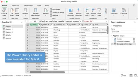
The Power Query Editor is a powerful tool in Excel that allows you to manipulate and analyze data. You can use the Power Query Editor to match multiple criteria by creating a custom formula.
To use the Power Query Editor, you need to go to the "Data" tab in the ribbon and click on "From Table/Range".
Then, you can select the range of cells that you want to manipulate and click on "OK".
In the Power Query Editor, you can create a custom formula by clicking on "Add Column" and then selecting "Custom Column".
For example, suppose you have a range of data in cells A1:C10, and you want to match multiple criteria to extract the sales value for a specific employee in a specific department.
Example Using Power Query Editor
| Name | Department | Sales |
|---|---|---|
| John | Sales | 100 |
| Jane | Marketing | 200 |
| John | Sales | 300 |
| Bob | Sales | 400 |
To match multiple criteria using the Power Query Editor, you can create a custom formula as follows:
= Table.SelectRows(Source, each [Name] = "John" and [Department] = "Sales")
This formula will return only the rows where the name is "John" and the department is "Sales".
Using the Advanced Filter
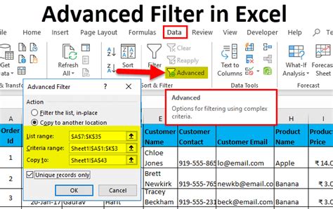
The Advanced Filter is a powerful feature in Excel that allows you to filter data based on multiple criteria. To use the Advanced Filter, you need to go to the "Data" tab in the ribbon and click on "Advanced".
Then, you can select the range of cells that you want to filter and click on "OK".
In the Advanced Filter dialog box, you can select the criteria range and the filter range.
For example, suppose you have a range of data in cells A1:C10, and you want to filter the data to show only the records where the value in column A is "John" and the value in column B is "Sales".
Example Using Advanced Filter
| Name | Department | Sales |
|---|---|---|
| John | Sales | 100 |
| Jane | Marketing | 200 |
| John | Sales | 300 |
| Bob | Sales | 400 |
To filter the data using the Advanced Filter, you can select the criteria range as A1:B10 and the filter range as A1:C10.
Then, you can click on "OK" to apply the filter.
The Advanced Filter will return only the records where the value in column A is "John" and the value in column B is "Sales".
Gallery of Excel Multiple Criteria
Excel Multiple Criteria Image Gallery




We hope this article has provided you with a comprehensive guide on how to match multiple criteria in Excel. Whether you are a beginner or an advanced user, these methods will help you to manipulate and analyze your data efficiently.
Remember to practice these methods to become proficient in using them. If you have any questions or need further clarification, please leave a comment below.
