
Vlookup Across Multiple Sheets in Excel: A Comprehensive Guide
Are you tired of searching for data across multiple sheets in Excel? Do you want to learn how to use the VLOOKUP function to retrieve data from multiple sheets? Look no further! In this article, we will explore five ways to VLOOKUP across multiple sheets in Excel. Whether you're a beginner or an advanced user, this guide will help you master the VLOOKUP function and take your Excel skills to the next level.
What is VLOOKUP?
Before we dive into the five ways to VLOOKUP across multiple sheets, let's quickly review what the VLOOKUP function is. VLOOKUP is a powerful function in Excel that allows you to search for a value in a table and return a corresponding value from another column. The syntax for the VLOOKUP function is:
VLOOKUP(lookup_value, table_array, col_index_num, [range_lookup])
Where:
- lookup_value is the value you want to search for
- table_array is the range of cells that contains the data you want to search
- col_index_num is the column number that contains the value you want to return
- [range_lookup] is an optional argument that specifies whether you want an exact match or an approximate match
Method 1: Using the VLOOKUP Function with Multiple Sheets
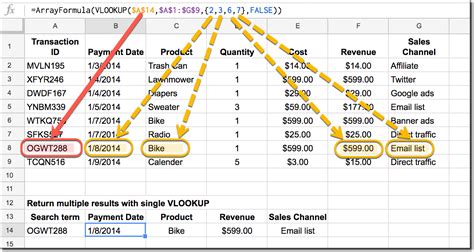
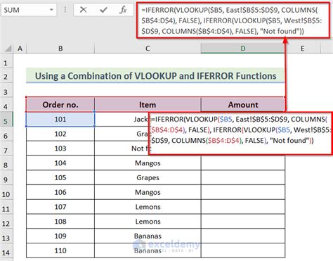
One way to VLOOKUP across multiple sheets is to use the VLOOKUP function with multiple sheet references. For example, let's say you have two sheets: "Sheet1" and "Sheet2". You want to search for a value in column A of Sheet1 and return the corresponding value in column B of Sheet2.
The formula would look like this:
=VLOOKUP(A2, Sheet1!A:B, 2, FALSE)
Where:
- A2 is the cell that contains the value you want to search for
- Sheet1!A:B is the range of cells that contains the data you want to search
- 2 is the column number that contains the value you want to return
- FALSE specifies an exact match
Step-by-Step Instructions
- Open your Excel workbook and select the cell where you want to display the result.
- Type the VLOOKUP formula, starting with the equals sign (=).
- Select the cell that contains the value you want to search for (A2).
- Select the range of cells that contains the data you want to search (Sheet1!A:B).
- Enter the column number that contains the value you want to return (2).
- Specify whether you want an exact match or an approximate match (FALSE).
- Press Enter to display the result.
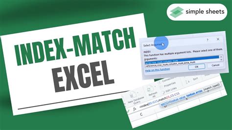
Method 2: Using the INDEX-MATCH Function
Another way to VLOOKUP across multiple sheets is to use the INDEX-MATCH function. This function is more flexible than VLOOKUP and allows you to search for a value in multiple columns.
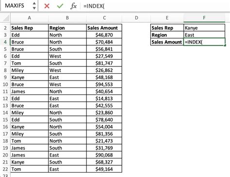
The formula would look like this:
=INDEX(Sheet2!B:B, MATCH(A2, Sheet1!A:A, 0))
Where:
- A2 is the cell that contains the value you want to search for
- Sheet1!A:A is the range of cells that contains the data you want to search
- Sheet2!B:B is the range of cells that contains the value you want to return
- 0 specifies an exact match
Step-by-Step Instructions
- Open your Excel workbook and select the cell where you want to display the result.
- Type the INDEX-MATCH formula, starting with the equals sign (=).
- Select the range of cells that contains the value you want to return (Sheet2!B:B).
- Select the cell that contains the value you want to search for (A2).
- Select the range of cells that contains the data you want to search (Sheet1!A:A).
- Specify whether you want an exact match or an approximate match (0).
- Press Enter to display the result.
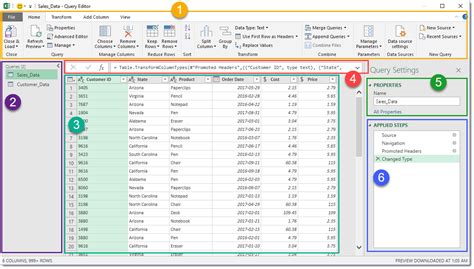
Method 3: Using Power Query
Power Query is a powerful tool in Excel that allows you to connect to multiple data sources and transform data. You can use Power Query to VLOOKUP across multiple sheets.
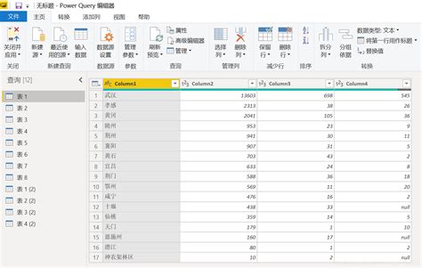
To use Power Query, follow these steps:
- Open your Excel workbook and go to the Data tab.
- Click on the New Query button and select From Other Sources.
- Select the range of cells that contains the data you want to search.
- Click on the Load button to load the data into Power Query.
- In the Power Query Editor, click on the Merge Queries button.
- Select the range of cells that contains the value you want to return.
- Click on the OK button to merge the queries.
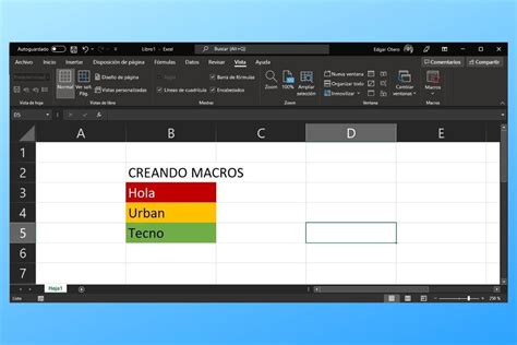
Method 4: Using Macros
Macros are a way to automate tasks in Excel using VBA code. You can use macros to VLOOKUP across multiple sheets.

To use macros, follow these steps:
- Open your Excel workbook and go to the Developer tab.
- Click on the Visual Basic button to open the Visual Basic Editor.
- In the Visual Basic Editor, click on the Insert button and select Module.
- Paste the following code into the module:
Sub VLOOKUP_Macro() Dim lookup_value As String Dim table_array As Range Dim col_index_num As Integer Dim range_lookup As Boolean
lookup_value = "A2"
table_array = Range("Sheet1!A:B")
col_index_num = 2
range_lookup = False

Range("C2").Value = Application.VLookup(lookup_value, table_array, col_index_num, range_lookup)
End Sub
- Click on the Run button to run the macro.
Method 5: Using Excel Formulas with Multiple Criteria
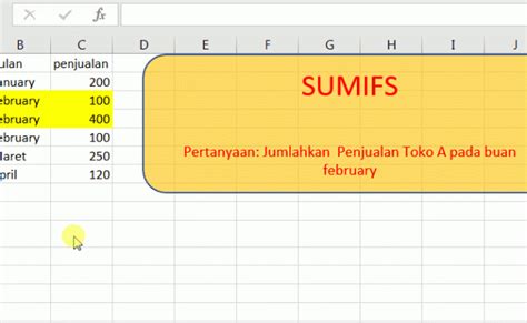
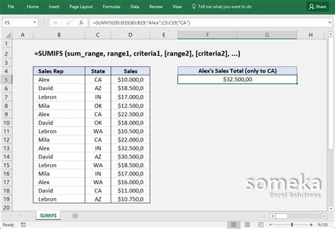
Another way to VLOOKUP across multiple sheets is to use Excel formulas with multiple criteria. You can use the SUMIFS function to search for a value in multiple columns.
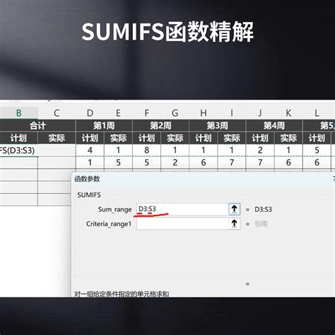
The formula would look like this:
=SUMIFS(Sheet2!B:B, Sheet1!A:A, A2, Sheet1!C:C, " Criteria")
Where:
- A2 is the cell that contains the value you want to search for
- Sheet1!A:A is the range of cells that contains the data you want to search
- Sheet2!B:B is the range of cells that contains the value you want to return
- Sheet1!C:C is the range of cells that contains the criteria
- "Criteria" is the criteria you want to apply
Step-by-Step Instructions
- Open your Excel workbook and select the cell where you want to display the result.
- Type the SUMIFS formula, starting with the equals sign (=).
- Select the range of cells that contains the value you want to return (Sheet2!B:B).
- Select the range of cells that contains the data you want to search (Sheet1!A:A).
- Select the cell that contains the value you want to search for (A2).
- Select the range of cells that contains the criteria (Sheet1!C:C).
- Enter the criteria you want to apply ("Criteria").
- Press Enter to display the result.
VLOOKUP Across Multiple Sheets Image Gallery

In conclusion, there are many ways to VLOOKUP across multiple sheets in Excel. Whether you use the VLOOKUP function, the INDEX-MATCH function, Power Query, macros, or Excel formulas with multiple criteria, you can easily retrieve data from multiple sheets. Remember to always use the correct syntax and to test your formulas to ensure they work correctly.