Intro
Master the art of calculating weighted averages in Google Sheets with ease. Learn how to use formulas and functions to assign different weights to data points, making complex calculations a breeze. Discover how to apply weighted averages to real-world scenarios, including grades, investments, and ratings, and make data-driven decisions with confidence.
Calculating weighted averages is a common task in various fields, such as finance, education, and data analysis. Google Sheets provides an efficient way to perform this calculation, and in this article, we will explore the different methods to calculate weighted averages in Google Sheets.
What is a Weighted Average?
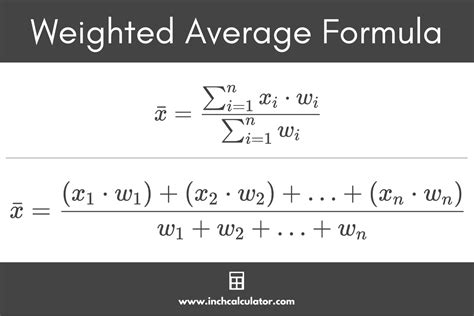
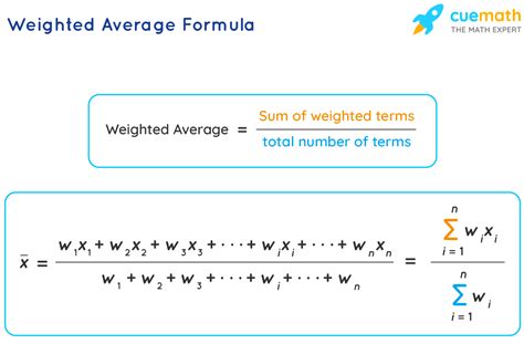
A weighted average is a type of average that takes into account the relative importance or weight of each value in a dataset. Unlike a simple average, which assigns equal weight to each value, a weighted average assigns a specific weight to each value based on its relative importance.
Why Use Weighted Averages?
Weighted averages are useful in situations where some values have more importance or influence than others. For example, in finance, a company's overall performance may be influenced more by its high-performing departments than its low-performing ones. In education, a student's overall grade may be influenced more by their performance in critical subjects than elective ones.
Method 1: Using the AVERAGE.WEIGHTED Function
Google Sheets provides a built-in function called AVERAGE.WEIGHTED, which calculates the weighted average of a range of values. The syntax for this function is:
AVERAGE.WEIGHTED(values, weights)
Where:
valuesis the range of values to be averagedweightsis the range of weights corresponding to each value

Example:
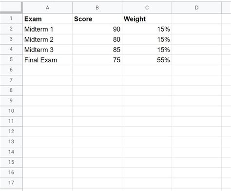
Suppose we have a dataset of exam scores and corresponding weights for each subject.
| Subject | Score | Weight |
|---|---|---|
| Math | 80 | 0.3 |
| Science | 90 | 0.4 |
| English | 70 | 0.3 |
To calculate the weighted average, we can use the AVERAGE.WEIGHTED function as follows:
=AVERAGE.WEIGHTED(B2:B4, C2:C4)
Where B2:B4 is the range of scores and C2:C4 is the range of weights.
Method 2: Using SUMPRODUCT and SUM
Another way to calculate weighted averages in Google Sheets is to use the SUMPRODUCT and SUM functions. The syntax for this method is:
=SUMPRODUCT(values, weights) / SUM(weights)
Where:
valuesis the range of values to be averagedweightsis the range of weights corresponding to each value
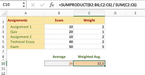
Example:
Using the same dataset as before, we can calculate the weighted average as follows:
=SUMPRODUCT(B2:B4, C2:C4) / SUM(C2:C4)
Where B2:B4 is the range of scores and C2:C4 is the range of weights.
Method 3: Using Arrays
Google Sheets also allows us to calculate weighted averages using arrays. The syntax for this method is:
=ArrayFormula(SUM(values * weights) / SUM(weights))
Where:
valuesis the range of values to be averagedweightsis the range of weights corresponding to each value
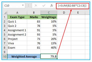
Example:
Using the same dataset as before, we can calculate the weighted average as follows:
=ArrayFormula(SUM(B2:B4 * C2:C4) / SUM(C2:C4))
Where B2:B4 is the range of scores and C2:C4 is the range of weights.
Conclusion:
Calculating weighted averages in Google Sheets is a straightforward process that can be accomplished using various methods. The AVERAGE.WEIGHTED function provides a simple and efficient way to calculate weighted averages, while the SUMPRODUCT and SUM functions offer an alternative approach. Additionally, using arrays provides a flexible way to perform calculations with multiple values and weights. By understanding these methods, you can easily calculate weighted averages in Google Sheets and make informed decisions based on your data.
Weighted Average Image Gallery

