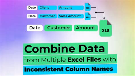
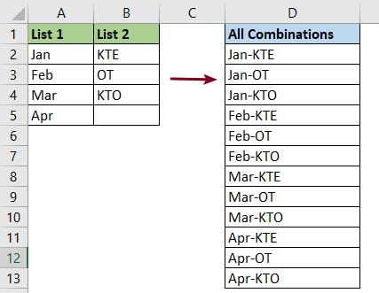
Combine Data In Excel From Multiple Worksheets Easily

Combining data in Excel from multiple worksheets can be a daunting task, especially when dealing with large datasets. However, with the right techniques and tools, it can be done easily and efficiently. In this article, we will explore the different methods to combine data from multiple worksheets in Excel, including using formulas, pivot tables, and Power Query.

Understanding the Importance of Combining Data

Before we dive into the methods, it's essential to understand why combining data from multiple worksheets is crucial. In many organizations, data is scattered across different worksheets, workbooks, or even databases. This can lead to data silos, making it difficult to get a comprehensive view of the data. By combining data from multiple worksheets, you can:

Get a unified view of your data
Identify patterns and trends
Make informed decisions
Improve data analysis and reporting

Method 1: Using Formulas to Combine Data

One of the simplest ways to combine data from multiple worksheets is by using formulas. You can use the VLOOKUP or INDEX-MATCH functions to retrieve data from one worksheet and display it in another.

Using VLOOKUP

The VLOOKUP function allows you to search for a value in a table and return a corresponding value from another column. To use VLOOKUP, follow these steps:

Select the cell where you want to display the combined data.
Enter the VLOOKUP formula, specifying the value you want to search for, the range of cells to search, and the column index of the value you want to return.
Press Enter to execute the formula.

Example: =VLOOKUP(A2,Sheet2!A:B,2,FALSE)

Using INDEX-MATCH

The INDEX-MATCH function is more flexible and powerful than VLOOKUP. To use INDEX-MATCH, follow these steps:

Select the cell where you want to display the combined data.
Enter the INDEX-MATCH formula, specifying the range of cells to search, the value you want to search for, and the column index of the value you want to return.
Press Enter to execute the formula.

Example: =INDEX(Sheet2!B:B,MATCH(A2,Sheet2!A:A,0))

Method 2: Using Pivot Tables to Combine Data

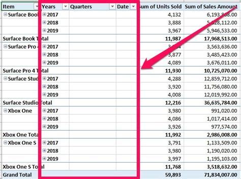
Pivot tables are a powerful tool in Excel that allows you to summarize and analyze large datasets. You can use pivot tables to combine data from multiple worksheets by following these steps:

Select the cell range that contains the data you want to combine.
Go to the "Insert" tab and click on "PivotTable."
Select a cell to place the pivot table and click "OK."
Drag the fields you want to combine to the "Row Labels" and "Values" areas.

Creating a Pivot Table

To create a pivot table, follow these steps:

Select the cell range that contains the data you want to combine.
Go to the "Insert" tab and click on "PivotTable."
Select a cell to place the pivot table and click "OK."
Drag the fields you want to combine to the "Row Labels" and "Values" areas.

Method 3: Using Power Query to Combine Data

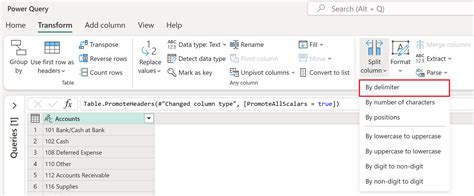
Power Query is a powerful tool in Excel that allows you to connect to different data sources, transform and shape the data, and load it into a worksheet. You can use Power Query to combine data from multiple worksheets by following these steps:

Go to the "Data" tab and click on "New Query."
Select "From Other Sources" and click on "From Microsoft Query."
Select the worksheets you want to combine and click "OK."
Use the Power Query Editor to transform and shape the data.

Using Power Query Editor

The Power Query Editor is a powerful tool that allows you to transform and shape the data. To use the Power Query Editor, follow these steps:

Go to the "Data" tab and click on "New Query."
Select "From Other Sources" and click on "From Microsoft Query."
Select the worksheets you want to combine and click "OK."
Use the Power Query Editor to transform and shape the data.

Gallery of Excel Data Combination

Excel Data Combination Gallery

Conclusion

Combining data in Excel from multiple worksheets can be a challenging task, but with the right techniques and tools, it can be done easily and efficiently. By using formulas, pivot tables, and Power Query, you can combine data from multiple worksheets and get a unified view of your data. Whether you're a beginner or an advanced user, this article has provided you with the necessary skills to combine data in Excel like a pro. So, go ahead and give it a try!

What's Your Experience with Combining Data in Excel?

We'd love to hear about your experience with combining data in Excel. Share your thoughts, tips, and tricks in the comments section below. If you have any questions or need further clarification on any of the methods discussed in this article, feel free to ask.