Comparing columns in Excel is a common task that can be accomplished using various methods, depending on the desired outcome. Whether you're looking to identify matches, highlight differences, or perform more complex operations, Excel provides a range of tools and functions to make the process efficient.
Finding matches between two columns is a fundamental operation in data analysis. It allows you to compare lists, verify data integrity, and even perform tasks like data deduplication or data merging. Excel offers several approaches to compare columns for matches, from simple formulas to more advanced techniques involving pivot tables or VBA macros.
Understanding the Need to Compare Columns
Before diving into the methods, it's essential to understand why comparing columns is important. In data analysis, comparing lists or columns can help in:
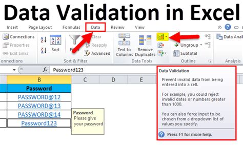
- Data Validation: Verifying if data entered in one column matches another.
- Data Merging: Combining data from two or more columns based on matching criteria.
- Data Deduplication: Identifying and removing duplicate entries across columns.
Basic Methods for Comparing Columns
Excel provides several basic methods to compare columns, including using formulas, conditional formatting, and the VLOOKUP function.
Using Formulas
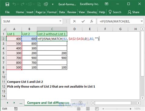
One of the simplest ways to compare two columns (A and B) is by using a formula in a new column. For example, you can use:
=IF(A1=B1, "Match", "No Match")
This formula checks if the values in cells A1 and B1 are the same. If they are, it returns "Match"; otherwise, it returns "No Match."
Conditional Formatting
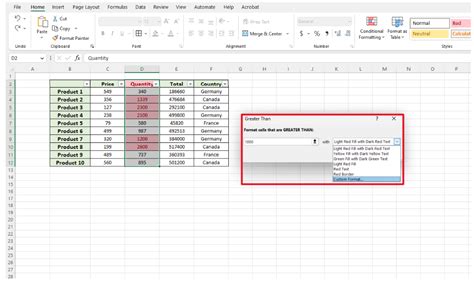
Conditional formatting allows you to highlight cells based on specific conditions. To highlight matches between two columns:
- Select the cells in one of the columns.
- Go to Home > Conditional Formatting > New Rule.
- Choose "Use a formula to determine which cells to format."
- Enter a formula like
=A1=B1(assuming you're comparing columns A and B starting from row 1). - Click "Format" to choose a format, then click "OK."
VLOOKUP Function
The VLOOKUP function can also be used to compare values and return a match from another column. The basic syntax is:
VLOOKUP(lookup_value, table_array, col_index_num, [range_lookup])
For example, to find a match from column A in column B and return the corresponding value from column C:
=VLOOKUP(A2, B:C, 2, FALSE)
Advanced Techniques
For more complex comparisons or when dealing with large datasets, you might need to employ advanced techniques.
Using INDEX and MATCH Functions
A more flexible and powerful alternative to VLOOKUP is combining the INDEX and MATCH functions. This method allows for more flexibility in the table structure and can handle larger datasets more efficiently.
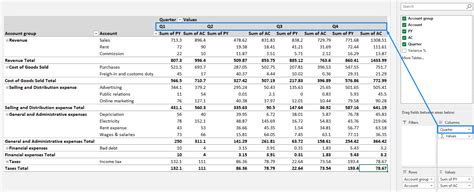
Pivot Tables
Pivot tables can also be used to compare and summarize data from multiple columns. They are particularly useful for analyzing large datasets and can help in identifying matches based on multiple criteria.
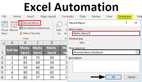
VBA Macros
For very complex operations or repetitive tasks, creating a VBA macro can automate the process of comparing columns and performing actions based on the results.
Best Practices
- Ensure Data Consistency: Before comparing columns, make sure the data is in a consistent format to avoid false negatives.
- Use Absolute References: When using formulas across different worksheets or workbooks, consider using absolute references to avoid errors.
- Test on a Small Scale: Before applying any method to a large dataset, test it on a small sample to ensure it works as expected.
Encouragement for Engagement
Comparing columns in Excel is a fundamental skill that can greatly enhance your productivity and data analysis capabilities. Whether you're just starting out with Excel or are a seasoned user, mastering these techniques can open up new possibilities for data manipulation and analysis. Share your favorite methods for comparing columns in Excel, or ask for help with a specific scenario you're facing. Your insights can help others in the community tackle similar challenges.

Gallery of Excel Column Comparison Techniques
