
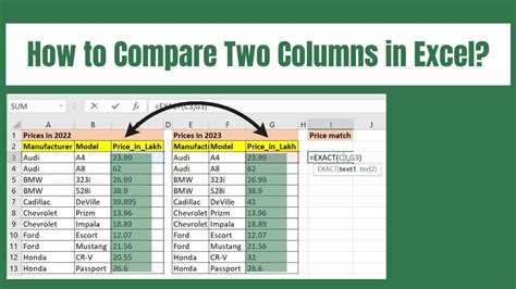
Comparing columns in Excel is a common task that can be useful in various scenarios, such as data analysis, data cleaning, and data visualization. Excel provides several methods to compare columns, each with its own strengths and limitations. In this article, we will explore five ways to compare columns in Excel.
Why Compare Columns in Excel?

Comparing columns in Excel can help you identify differences, similarities, and patterns in your data. It can also help you to:
- Identify duplicates or unique values
- Validate data entry
- Perform data quality checks
- Analyze data trends
- Make informed business decisions
Method 1: Using the IF Function
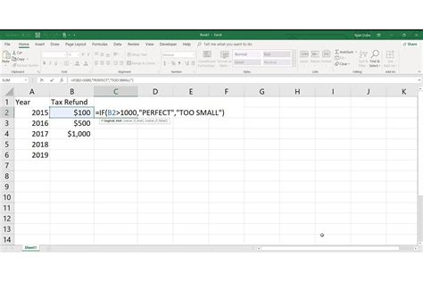
The IF function is a simple and effective way to compare two columns in Excel. The syntax for the IF function is:
IF(logical_test, [value_if_true], [value_if_false])
For example, suppose you want to compare two columns, A and B, and return "Match" if the values are the same and "No Match" if they are different. You can use the following formula:
=IF(A1=B1, "Match", "No Match")
Example:
| Column A | Column B | Comparison |
|---|---|---|
| Apple | Apple | Match |
| Banana | Orange | No Match |
| Cherry | Cherry | Match |
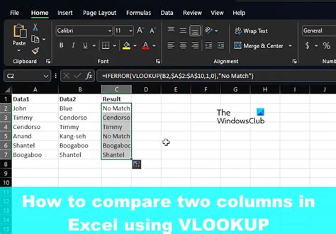
Method 2: Using the VLOOKUP Function
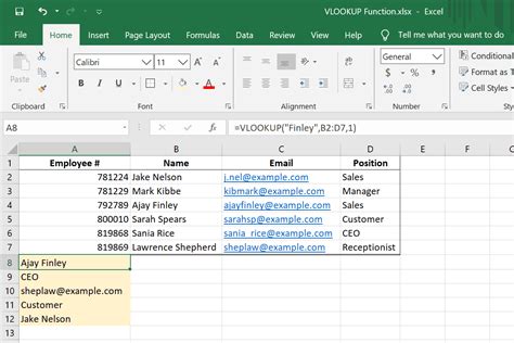
The VLOOKUP function is another powerful way to compare columns in Excel. The syntax for the VLOOKUP function is:
VLOOKUP(lookup_value, table_array, col_index_num, [range_lookup])
For example, suppose you want to compare two columns, A and B, and return the value in column C if the values in columns A and B match. You can use the following formula:
=VLOOKUP(A1, B:C, 2, FALSE)
Example:
| Column A | Column B | Column C |
|---|---|---|
| Apple | Apple | Red |
| Banana | Orange | Yellow |
| Cherry | Cherry | Pink |
Method 3: Using Conditional Formatting
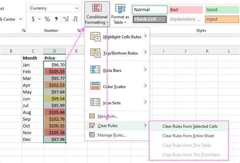
Conditional formatting is a great way to visually compare columns in Excel. You can use conditional formatting to highlight cells that match or do not match between two columns.
For example, suppose you want to highlight cells in column A that match cells in column B. You can use the following steps:
- Select the range of cells in column A.
- Go to the Home tab in the ribbon.
- Click on Conditional Formatting.
- Select "New Rule".
- Select "Use a formula to determine which cells to format".
- Enter the formula: =A1=B1
- Click on Format.
- Select a formatting option, such as fill color or font color.
Example:
| Column A | Column B |
|---|---|
| Apple | Apple |
| Banana | Orange |
| Cherry | Cherry |
Method 4: Using Power Query
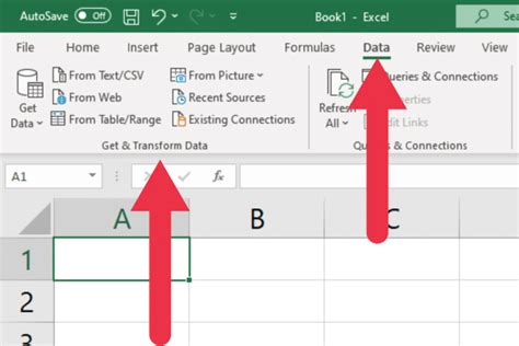
Power Query is a powerful tool in Excel that allows you to compare columns and perform data analysis. You can use Power Query to compare two columns and return the differences.
For example, suppose you want to compare two columns, A and B, and return the differences. You can use the following steps:
- Go to the Data tab in the ribbon.
- Click on From Table/Range.
- Select the range of cells in column A.
- Click on Load.
- Go to the Home tab in the ribbon.
- Click on Merge Queries.
- Select the range of cells in column B.
- Click on Merge.
Example:
| Column A | Column B | Differences |
|---|---|---|
| Apple | Apple | |
| Banana | Orange | Banana |
| Cherry | Cherry |
Method 5: Using the FILTER Function
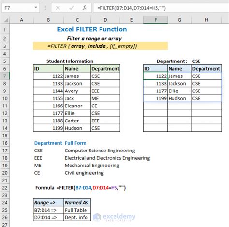
The FILTER function is a new function in Excel that allows you to compare columns and return the filtered results. The syntax for the FILTER function is:
FILTER(array, include, [if_empty])
For example, suppose you want to compare two columns, A and B, and return the values in column A that match the values in column B. You can use the following formula:
=FILTER(A:A, A:A=B:B)
Example:
| Column A | Column B | Filtered Results |
|---|---|---|
| Apple | Apple | Apple |
| Banana | Orange | |
| Cherry | Cherry | Cherry |
Column Comparison Image Gallery


In conclusion, comparing columns in Excel can be a useful task in various scenarios. The five methods discussed in this article, using the IF function, VLOOKUP function, conditional formatting, Power Query, and FILTER function, can help you to compare columns and achieve your desired results. Whether you are a beginner or an advanced user, these methods can help you to work more efficiently and effectively in Excel.