
The ability to filter data is an essential feature in data analysis, and Microsoft Excel provides an excellent tool for this purpose - the drop-down list filter. In this article, we will explore the different ways to use Excel's drop-down list filter to simplify your data analysis tasks.
Using a drop-down list filter in Excel allows you to quickly narrow down large datasets to specific subsets of data, making it easier to analyze and visualize your data. Whether you're working with sales data, customer information, or inventory management, the drop-down list filter is an indispensable tool for anyone who works with data in Excel.
Benefits of Using Excel Drop Down List Filter
Before we dive into the different ways to use the drop-down list filter, let's first look at the benefits of using this feature:
- Simplifies data analysis: The drop-down list filter allows you to quickly narrow down large datasets to specific subsets of data, making it easier to analyze and visualize your data.
- Saves time: By using the drop-down list filter, you can avoid having to manually sort and filter your data, saving you time and effort.
- Improves data accuracy: The drop-down list filter helps to reduce errors by ensuring that you're only looking at the data that's relevant to your analysis.
1. Filtering Data with a Single Drop-Down List
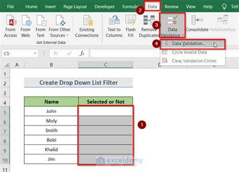
The most basic way to use the drop-down list filter is to filter data with a single drop-down list. To do this, select the cell range that you want to filter, go to the "Data" tab in the ribbon, and click on the "Filter" button. Then, click on the drop-down arrow next to the column header that you want to filter.
In the drop-down menu, you can select the specific value that you want to filter by. For example, if you're filtering sales data by region, you can select "North" from the drop-down menu to only show sales data for the North region.
2. Filtering Data with Multiple Drop-Down Lists
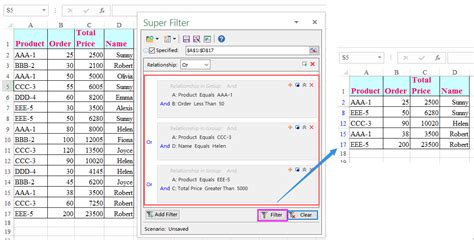
You can also use multiple drop-down lists to filter data. To do this, select the cell range that you want to filter, go to the "Data" tab in the ribbon, and click on the "Filter" button. Then, click on the drop-down arrow next to each column header that you want to filter.

In the drop-down menus, you can select the specific values that you want to filter by. For example, if you're filtering sales data by region and product category, you can select "North" from the region drop-down menu and "Electronics" from the product category drop-down menu to only show sales data for electronics in the North region.
3. Using Drop-Down Lists to Filter Data with Formulas
You can also use drop-down lists to filter data with formulas. To do this, select the cell range that you want to filter, go to the "Data" tab in the ribbon, and click on the "Filter" button. Then, click on the drop-down arrow next to the column header that you want to filter.
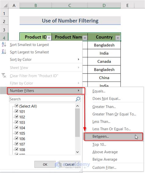
In the drop-down menu, you can select the specific formula that you want to use to filter your data. For example, if you're filtering sales data by total sales amount, you can select "Greater than 1000" from the drop-down menu to only show sales data with a total sales amount greater than 1000.
4. Creating a Dynamic Drop-Down List Filter
You can also create a dynamic drop-down list filter that updates automatically when you add new data to your dataset. To do this, select the cell range that you want to filter, go to the "Data" tab in the ribbon, and click on the "Filter" button. Then, click on the drop-down arrow next to the column header that you want to filter.
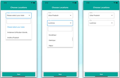
In the drop-down menu, you can select the specific value that you want to filter by. For example, if you're filtering sales data by region, you can select "North" from the drop-down menu to only show sales data for the North region. When you add new data to your dataset, the drop-down list filter will automatically update to include the new values.
5. Using Drop-Down Lists to Filter Data with PivotTables
Finally, you can use drop-down lists to filter data with PivotTables. To do this, select the cell range that you want to filter, go to the "Insert" tab in the ribbon, and click on the "PivotTable" button. Then, select the specific value that you want to filter by from the drop-down menu.
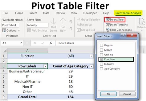
In the drop-down menu, you can select the specific value that you want to filter by. For example, if you're filtering sales data by region, you can select "North" from the drop-down menu to only show sales data for the North region.
Gallery of Excel Drop Down List Filter Examples
Excel Drop Down List Filter Image Gallery


In conclusion, the drop-down list filter is a powerful tool in Excel that can simplify your data analysis tasks. By using the different methods outlined in this article, you can use the drop-down list filter to filter data with single or multiple drop-down lists, use formulas to filter data, create dynamic drop-down list filters, and use drop-down lists to filter data with PivotTables.