5 Ways To Highlight In Excel If Greater Than

Highlighting cells in Excel based on specific conditions can greatly enhance the visual appeal and readability of your data. One common requirement is to highlight cells if their values are greater than a certain threshold. Excel's Conditional Formatting feature makes this task straightforward and powerful. Here's how you can use it to highlight cells that are greater than a specific value.

Using Conditional Formatting

Conditional Formatting is Excel's built-in feature for highlighting cells based on various conditions, including numerical values, formulas, and formatting.

Step 1: Select the Range

To start, select the range of cells you want to apply the formatting to. This can be a single column, multiple columns, or even the entire spreadsheet, depending on your needs.

Step 2: Go to Conditional Formatting

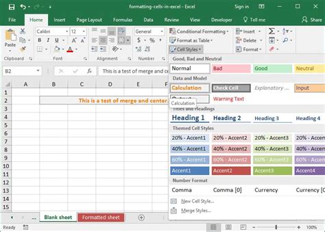
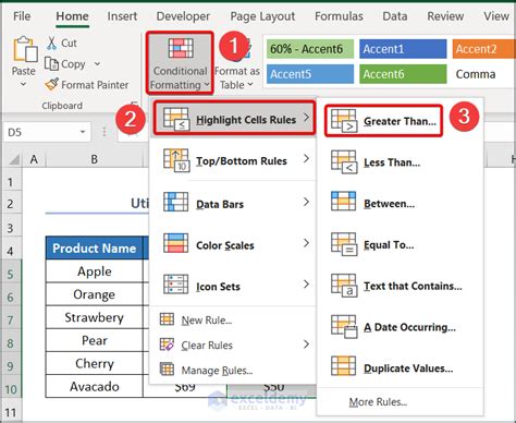
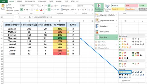
Navigate to the "Home" tab in the Excel ribbon. In the "Styles" group, click on "Conditional Formatting."

Step 3: Select "Highlight Cells Rules"

From the dropdown menu, select "Highlight Cells Rules." This option allows you to specify conditions based on cell values, such as greater than, less than, between, or equal to.

Step 4: Choose "Greater Than"

In the "Highlight Cells Rules" menu, click on "Greater Than." This option will highlight cells that contain values greater than the value you specify.

Step 5: Set the Value and Format

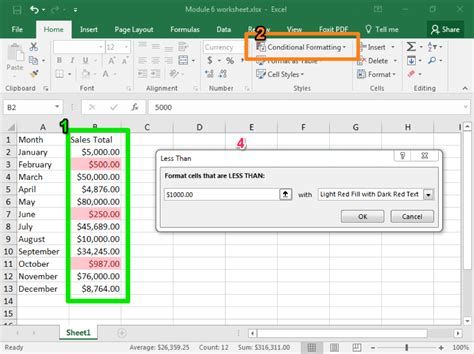
In the "Greater Than" dialog box, enter the value you want to compare the cell values against. You can also choose how you want the highlighted cells to look by selecting a format from the dropdown menu or creating a custom format.

Step 6: Apply the Formatting

Click "OK" to apply the formatting. Excel will immediately highlight the cells in your selected range that meet the condition (i.e., have values greater than the specified value).

Example: Highlighting Sales Greater Than $1000

Suppose you have a list of sales figures in column A and you want to highlight all sales greater than $1000.

1. Select the range A1:A100 (assuming your sales figures are listed from A1 to A100).
2. Go to "Home" > "Conditional Formatting" > "Highlight Cells Rules" > "Greater Than."
3. In the "Greater Than" dialog, enter 1000 as the value.
4. Choose a highlight format, such as green fill.
5. Click "OK."

Immediately, all sales figures greater than $1000 in the selected range will be highlighted in green.

Using Formulas in Conditional Formatting

For more complex conditions or comparisons, you can use formulas directly within Conditional Formatting.

Step 1: Select the Range

Select the range of cells you want to format.

Step 2: Go to Conditional Formatting

Navigate to "Home" > "Conditional Formatting" > "New Rule."

Step 3: Use a Formula

Select "Use a formula to determine which cells to format."

Step 4: Enter the Formula

In the formula box, enter your condition. For example, to highlight cells in column A where the value is greater than the average of the column, you might use =A1>AVERAGE($A:$A).

Step 5: Format Values

Click "Format" to choose the formatting style.

Step 6: Apply the Rule

Click "OK" to apply the rule.

Excel will highlight the cells based on the formula you provided.

Example: Highlighting Above Average Scores

If you have a list of scores in column B and you want to highlight any score that is above the average score:

1. Select the range B1:B100.
2. Go to "Home" > "Conditional Formatting" > "New Rule."
3. Choose "Use a formula to determine which cells to format."
4. Enter =B1>AVERAGE($B:$B) as the formula.
5. Click "Format" and choose a format.
6. Click "OK."

All scores in column B that are higher than the average will be highlighted.

Dynamic Formatting with Formulas

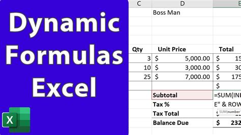
For dynamic and more flexible formatting, formulas can be adjusted based on cell references or other inputs.

Example: Highlighting Cells Based on User Input

If you want to highlight cells in a range based on a user-input threshold:

1. Place the threshold value in a specific cell, say cell D1.
2. Select the range you want to format.
3. Go to "Home" > "Conditional Formatting" > "New Rule."
4. Use the formula =A1>$D$1 (assuming your range starts in A1 and your threshold value is in D1).
5. Format as desired and click "OK."

This setup allows the user to change the threshold value in cell D1, and the formatting will automatically adjust.

Gallery of Excel Conditional Formatting Examples

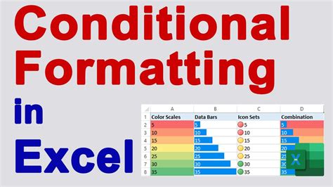
Conditional Formatting in Excel

Conclusion

Excel's Conditional Formatting is a powerful tool for data visualization and analysis. By highlighting cells based on specific conditions, such as values greater than a certain threshold, you can quickly identify trends, outliers, and areas of interest within your data. Whether you're using built-in rules or creating custom formulas, Conditional Formatting can significantly enhance your ability to understand and communicate insights from your data.

Feel free to ask any questions or share your experiences with Conditional Formatting in the comments below!