Excel Formula: Return Value Based On Two Criteria Match

When working with data in Excel, there are often instances where you need to find and return a value based on multiple criteria. While Excel's built-in functions like VLOOKUP and INDEX-MATCH are powerful tools for searching and retrieving data, they are typically designed to work with a single criterion. However, with a combination of functions or by using more advanced formulas, you can easily search and return values based on two or more criteria.

Understanding the Problem

Imagine you have a dataset that includes names, ages, and departments of employees within a company. You want to find the age of a specific employee who works in a particular department. In this scenario, you have two criteria: the name of the employee and the department they work in.

Using INDEX-MATCH for Multiple Criteria

One of the most efficient ways to return a value based on multiple criteria is by using the INDEX-MATCH combination. This method involves creating an array formula that can handle multiple criteria.

Assuming your data is structured as follows:

Name	Department	Age
John	Sales	32
Mary	Marketing	29
David	Sales	41

To find the age of John in the Sales department, you can use the following formula:

=INDEX(C:C, MATCH(1, (A:A="John") * (B:B="Sales"), 0))

This formula works as follows:

A:A="John" and B:B="Sales" create arrays of TRUE/FALSE values based on whether the name is John and the department is Sales, respectively.
Multiplying these arrays together gives another array where only the positions that match both criteria are TRUE (and thus 1 when multiplied), while all other positions are FALSE (and thus 0).
The MATCH function then finds the position of the first 1 in this array (which corresponds to the row where both criteria are met) and uses it as the row number for the INDEX function to return the age.

Using VLOOKUP with Multiple Criteria

While VLOOKUP is not as versatile as INDEX-MATCH for multiple criteria searches, it can be adapted by creating a helper column that combines the criteria.

Combining Criteria in a Helper Column

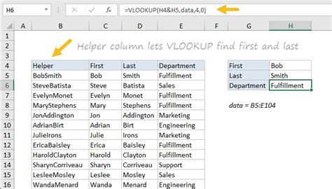
To use VLOOKUP, you can create a helper column that concatenates the name and department. For example, if your data is in columns A (Name), B (Department), and C (Age), you can create a helper column in D as follows:

Name	Department	Age	Helper (D)
John	Sales	32	JohnSales
Mary	Marketing	29	MaryMarketing
David	Sales	41	DavidSales

The formula for the helper column (in D2, for example) is:

=A2&B2

Then, you can use VLOOKUP to find the age based on the combined criteria:

=VLOOKUP("JohnSales", D:C, 2, FALSE)

This formula looks for "JohnSales" in the helper column (D) and returns the corresponding age from column C.

Using FILTER Function (Excel 365 and Later)

Excel FILTER Function for Multiple Criteria

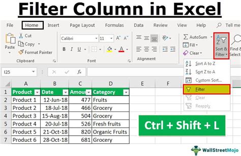
For users with Excel 365 or later versions, the FILTER function provides a straightforward way to filter data based on multiple criteria.

Assuming the same dataset:

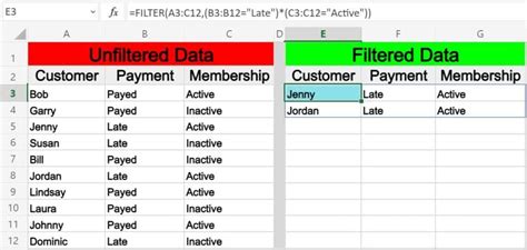
=FILTER(C:C, (A:A="John") * (B:B="Sales"))

This formula filters column C (Age) based on the conditions that the name in column A is "John" and the department in column B is "Sales".

Conclusion and Next Steps

Finding and returning values based on multiple criteria in Excel can significantly enhance your data analysis capabilities. By mastering the INDEX-MATCH combination, adapting VLOOKUP with helper columns, or utilizing the FILTER function in newer Excel versions, you can efficiently navigate and extract insights from complex datasets. Practice these methods with different datasets and explore how they can be applied to various data analysis tasks.