In the world of statistics and data analysis, the p-value plays a crucial role in determining the significance of results. Excel, being a powerful tool for data analysis, offers several ways to calculate the p-value. In this article, we will explore five easy ways to find the p-value in Excel.
Understanding the P-Value
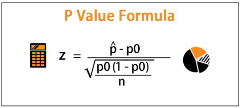
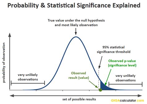
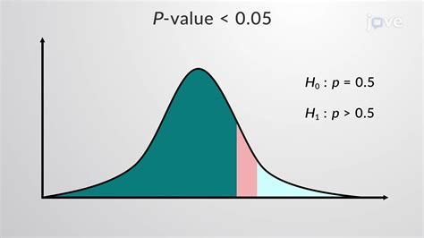
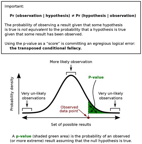
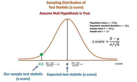
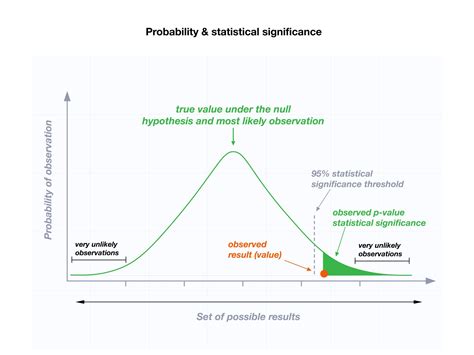
Before we dive into the methods, let's quickly understand what a p-value is. The p-value, or probability value, is a measure of the probability of observing a result at least as extreme as the one you obtained, assuming that the null hypothesis is true. In simpler terms, it helps you determine whether your results are due to chance or if they are statistically significant.
Method 1: Using the T.TEST Function
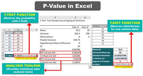
One of the easiest ways to calculate the p-value in Excel is by using the T.TEST function. This function is used to calculate the probability associated with a student's t-test.

To use the T.TEST function, follow these steps:
- Select the cell where you want to display the p-value.
- Type
=T.TEST(array1, array2, tails, type)and press Enter. - Array1 and array2 are the ranges of data you want to compare.
- Tails specify whether you want a one-tailed or two-tailed test.
- Type specifies the type of t-test you want to perform.
Method 2: Using the Z.TEST Function
Another way to calculate the p-value in Excel is by using the Z.TEST function. This function is used to calculate the probability associated with a z-test.
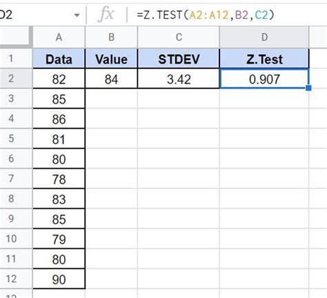
To use the Z.TEST function, follow these steps:
- Select the cell where you want to display the p-value.
- Type
=Z.TEST(array1, x, sigma)and press Enter. - Array1 is the range of data you want to compare.
- X is the value you want to test.
- Sigma is the standard deviation of the population.
Method 3: Using the F.TEST Function
If you're working with two samples and want to compare their variances, you can use the F.TEST function to calculate the p-value.
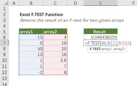
To use the F.TEST function, follow these steps:
- Select the cell where you want to display the p-value.
- Type
=F.TEST(array1, array2)and press Enter. - Array1 and array2 are the ranges of data you want to compare.
Method 4: Using the CHISQ.TEST Function
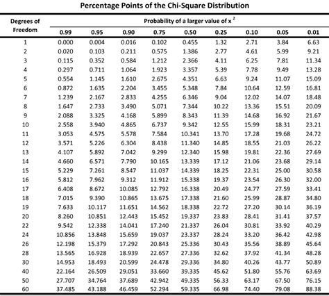
If you're working with categorical data and want to perform a chi-squared test, you can use the CHISQ.TEST function to calculate the p-value.

To use the CHISQ.TEST function, follow these steps:
- Select the cell where you want to display the p-value.
- Type
=CHISQ.TEST(actual_range, expected_range)and press Enter. - Actual_range is the range of actual frequencies.
- Expected_range is the range of expected frequencies.
Method 5: Using the Analysis ToolPak
Finally, you can use the Analysis ToolPak in Excel to calculate the p-value. The Analysis ToolPak is an add-in that provides a range of statistical tools, including t-tests, z-tests, and chi-squared tests.
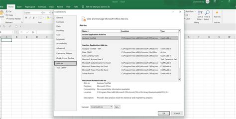
To use the Analysis ToolPak, follow these steps:
- Go to the Data tab in the ribbon.
- Click on Data Analysis.
- Select the type of test you want to perform.
- Follow the prompts to enter your data and select the options you want.
- Click OK to calculate the p-value.
Gallery of P-Value Images
P-Value Images

Conclusion
In this article, we explored five easy ways to find the p-value in Excel. Whether you're using the T.TEST function, Z.TEST function, F.TEST function, CHISQ.TEST function, or the Analysis ToolPak, Excel provides a range of tools to help you calculate the p-value. By understanding the different methods and formulas, you can make informed decisions about your data and improve your statistical analysis.
