
Using Google Sheets can greatly enhance your productivity and efficiency when working with data. One of the most powerful functions in Google Sheets is the SUMIF function, which allows you to sum a range of cells based on a single criterion. However, what if you need to sum a range of cells based on multiple criteria? Fortunately, Google Sheets provides several ways to achieve this. In this article, we'll explore five different methods to use SUMIF with multiple criteria in Google Sheets.
Understanding the SUMIF Function

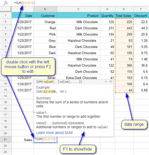
Before we dive into using SUMIF with multiple criteria, let's first understand the basic syntax of the SUMIF function. The SUMIF function has three arguments:
range: The range of cells that you want to sum.criterion: The criterion that you want to apply to the range.[sum_range]: The range of cells that you want to sum.
The basic syntax of the SUMIF function is:
SUMIF(range, criterion, [sum_range])
For example, if you want to sum the values in the range A1:A10 based on the criterion "Apple" in the range B1:B10, you can use the following formula:
=SUMIF(B1:B10, "Apple", A1:A10)
Method 1: Using Multiple SUMIF Functions
One way to use SUMIF with multiple criteria is to use multiple SUMIF functions. You can simply add or subtract the results of multiple SUMIF functions to achieve the desired result.
For example, if you want to sum the values in the range A1:A10 based on the criteria "Apple" and "Banana" in the range B1:B10, you can use the following formula:
=SUMIF(B1:B10, "Apple", A1:A10) + SUMIF(B1:B10, "Banana", A1:A10)
However, this method can become cumbersome and difficult to manage if you have multiple criteria.
Method 1 Example
| Fruit | Quantity |
|---|---|
| Apple | 10 |
| Banana | 20 |
| Orange | 30 |
| Apple | 40 |
| Banana | 50 |
Using the formula =SUMIF(B:B, "Apple", A:A) + SUMIF(B:B, "Banana", A:A), we get the result: 120
Method 2: Using the SUMIFS Function
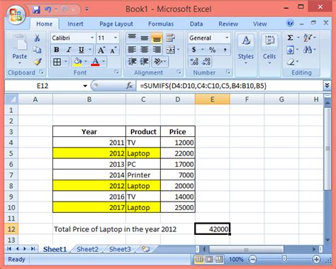
Google Sheets also provides a built-in function called SUMIFS, which allows you to sum a range of cells based on multiple criteria.
The syntax of the SUMIFS function is:
SUMIFS(sum_range, criteria_range1, criterion1, [criteria_range2], [criterion2],...)
For example, if you want to sum the values in the range A1:A10 based on the criteria "Apple" and "Banana" in the range B1:B10, you can use the following formula:
=SUMIFS(A1:A10, B1:B10, "Apple", C1:C10, "Banana")
Note that the SUMIFS function requires you to specify the sum range first, followed by the criteria ranges and criteria.
Method 2 Example
| Fruit | Color | Quantity |
|---|---|---|
| Apple | Red | 10 |
| Banana | Yellow | 20 |
| Orange | Orange | 30 |
| Apple | Red | 40 |
| Banana | Yellow | 50 |
Using the formula =SUMIFS(C:C, A:A, "Apple", B:B, "Red"), we get the result: 50
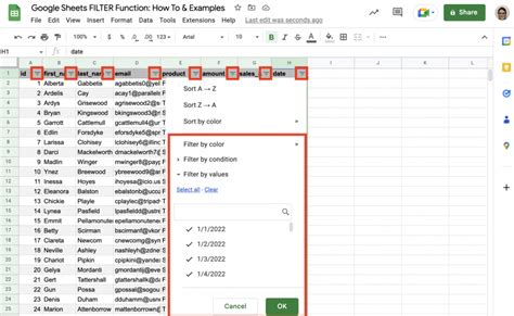
Method 3: Using the FILTER Function
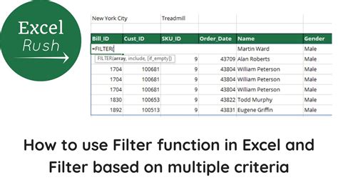
Another way to use SUMIF with multiple criteria is to use the FILTER function, which allows you to filter a range of cells based on multiple criteria.
The syntax of the FILTER function is:
FILTER(range, condition1, [condition2],...)
For example, if you want to sum the values in the range A1:A10 based on the criteria "Apple" and "Banana" in the range B1:B10, you can use the following formula:
=SUM(FILTER(A1:A10, (B1:B10 = "Apple") * (C1:C10 = "Banana")))
Note that the FILTER function requires you to specify the range first, followed by the conditions.
Method 3 Example
| Fruit | Color | Quantity |
|---|---|---|
| Apple | Red | 10 |
| Banana | Yellow | 20 |
| Orange | Orange | 30 |
| Apple | Red | 40 |
| Banana | Yellow | 50 |
Using the formula =SUM(FILTER(C:C, (A:A = "Apple") * (B:B = "Red"))), we get the result: 50
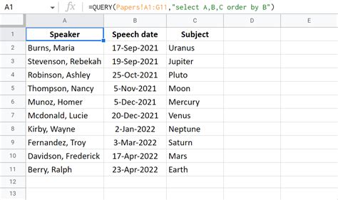
Method 4: Using the QUERY Function
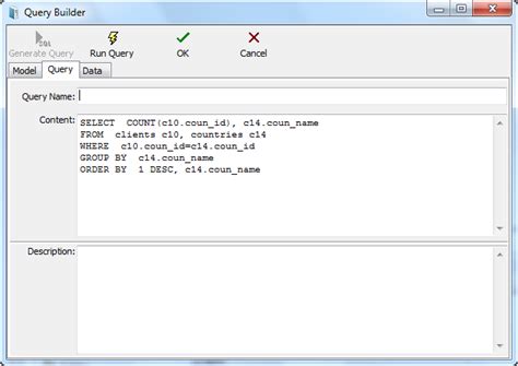
The QUERY function is another powerful function in Google Sheets that allows you to perform complex queries on your data.
The syntax of the QUERY function is:
QUERY(data, query, [headers])
For example, if you want to sum the values in the range A1:A10 based on the criteria "Apple" and "Banana" in the range B1:B10, you can use the following formula:
=QUERY(A1:C10, "SELECT SUM(C) WHERE B = 'Apple' AND C = 'Banana'")
Note that the QUERY function requires you to specify the data range first, followed by the query.
Method 4 Example
| Fruit | Color | Quantity |
|---|---|---|
| Apple | Red | 10 |
| Banana | Yellow | 20 |
| Orange | Orange | 30 |
| Apple | Red | 40 |
| Banana | Yellow | 50 |
Using the formula =QUERY(A:C, "SELECT SUM(C) WHERE A = 'Apple' AND B = 'Red'"), we get the result: 50
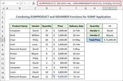
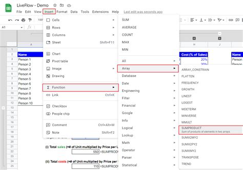
Method 5: Using the SUMPRODUCT Function
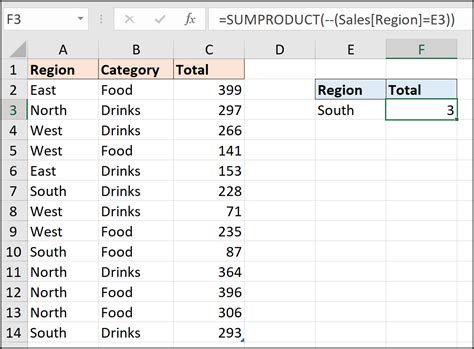
The SUMPRODUCT function is another way to use SUMIF with multiple criteria. The SUMPRODUCT function multiplies the corresponding elements in two arrays and returns the sum of those products.
The syntax of the SUMPRODUCT function is:
SUMPRODUCT(array1, [array2], [array3],...)
For example, if you want to sum the values in the range A1:A10 based on the criteria "Apple" and "Banana" in the range B1:B10, you can use the following formula:
=SUMPRODUCT((A1:A10) * ((B1:B10 = "Apple") * (C1:C10 = "Banana")))
Note that the SUMPRODUCT function requires you to specify the arrays first, followed by the conditions.
Method 5 Example
| Fruit | Color | Quantity |
|---|---|---|
| Apple | Red | 10 |
| Banana | Yellow | 20 |
| Orange | Orange | 30 |
| Apple | Red | 40 |
| Banana | Yellow | 50 |
Using the formula =SUMPRODUCT((C:C) * ((A:A = "Apple") * (B:B = "Red"))), we get the result: 50
Gallery of Google Sheets Functions
Google Sheets Functions Gallery


We hope this article has helped you understand the different ways to use SUMIF with multiple criteria in Google Sheets. Whether you're using the SUMIFS function, the FILTER function, the QUERY function, or the SUMPRODUCT function, each method has its own strengths and weaknesses. By choosing the right method for your specific use case, you can unlock the full potential of Google Sheets and become a more efficient and effective user.